램버트 문제(https://pasus.tistory.com/316)를 풀기 위한 알고리즘은 여러가지가 제안되어 있지만 여기서는 물리 정보 신경망(PINN, physics-informed neural network)을 이용하여 이 문제를 풀어보고자 한다. 수치 데이터는 이전 게시글(https://pasus.tistory.com/297)에서 사용했던 것을 다시 사용한다.
먼저 램버트 문제의 운동 방정식은 다음과 같다.
\[ \begin{align} \frac{d^2 \mathbf{r}}{dt^2 }+ \frac{\mu}{ \left( \sqrt{\mathbf{r} \cdot \mathbf{r}} \right)^3} \mathbf{r}=0 \tag{1} \end{align} \]
여기서 \(\mu\) 는 중력 파라미터, \(\mathbf{r}\) 은 관성 좌표계의 원점에서 질점까지의 위치벡터다. 식 (1)에서 속도 성분을 명시적으로 나타나게 표현할 수도 있다.
\[ \begin{align} & \frac{d \mathbf{r}}{dt} = \mathbf{v} \tag{2} \\ \\ & \frac{d \mathbf{v}}{dt}+ \frac{\mu}{ \left( \sqrt{\mathbf{r} \cdot \mathbf{r}} \right)^3} \mathbf{r}=0 \end{align} \]
식 (1)과 (2)는 동일한 식이지만 PINN으로 구현할 때는 차이가 있다. 식 (1)의 경우에는 2차 수치미분이 필요하지만 식 (2)의 경우에는 1차 수치미분이면 된다. 신경망의 학습 관점에서 보면 2차 미분 보다는 1차 미분 계산이 유리하므로 여기서는 식 (2)를 신경망으로 구현하고자 한다. 참고로 식 (1)로도 구현해 보니 별반 차이는 없었다.
PINN의 구조는 다음과 같다.
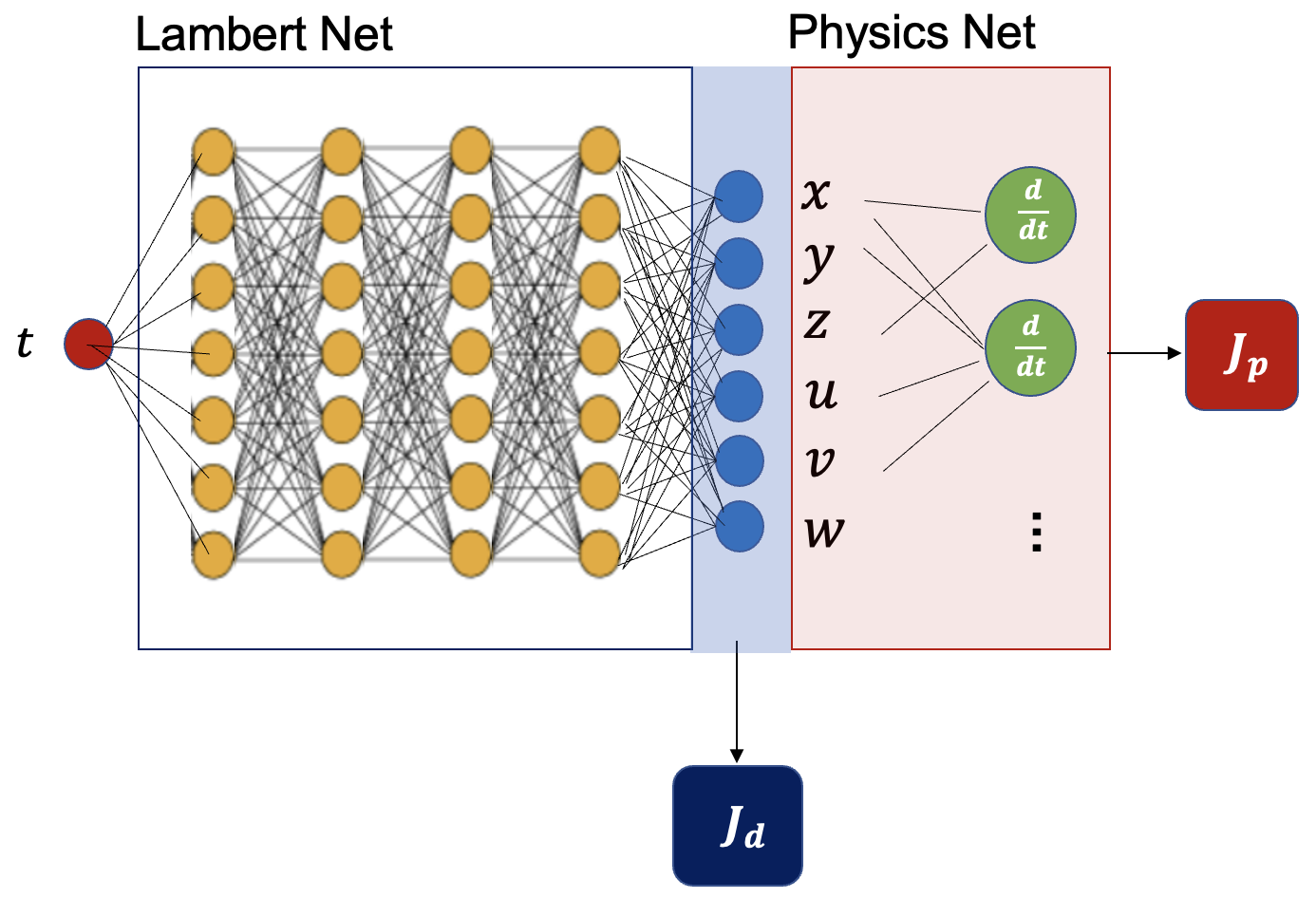
그림 왼쪽의 램버트 신경망은 입력이 시간인 \(t\) 이고 출력은 식 (2) 의 근사해인 \(\mathbf{r}=[x \ \ y \ \ z]^T \), \(\mathbf{v}=[u \ \ v \ \ w]^T\) 로 주어지는 완전연결 신경망이다. 신경망은 4개의 hidden layer로 구성되어 있으며 각 레이어는 10개의 뉴런을 갖는다. 활성함수로는 'tanh'를 사용했다.
class Lambert(Model):

    def __init__(self):
        super(Lambert, self).__init__()
        initializer = tf.keras.initializers.GlorotUniform
        self.h1 = Dense(10, activation='tanh', kernel_initializer=initializer)
        self.h2 = Dense(10, activation='tanh', kernel_initializer=initializer)
        self.h3 = Dense(10, activation='tanh', kernel_initializer=initializer)
        self.h4 = Dense(10, activation='tanh', kernel_initializer=initializer)
        self.out = Dense(6, activation='linear', kernel_initializer=initializer)

    def call(self, t):
        rv = self.h1(t) # time
        rv = self.h2(rv)
        rv = self.h3(rv)
        rv = self.h4(rv)
        rv = self.out(rv)

        x = rv[:, 0:1]
        y = rv[:, 1:2]
        z = rv[:, 2:3]
        u = rv[:, 3:4]
        v = rv[:, 4:5]
        w = rv[:, 5:6]

        return x, y, z, u, v, w
물리 신경망은 식 (2)의 미분방정식을 구현한 신경망으로서 Tensorflow 2의 자동미분 기능을 이용하여 구현했다.
    @tf.function
    def physics_net(self, t):
        x,y,z,u,v,w = self.lambert(t)
        x_t = tf.gradients(x, t)
        y_t = tf.gradients(y, t)
        z_t = tf.gradients(z, t)
        u_t = tf.gradients(u, t)
        v_t = tf.gradients(v, t)
        w_t = tf.gradients(w, t)

        r = tf.sqrt(x*x + y*y + z*z) + 0.00001
        r3 = r*r*r
        f1 = u_t + x/r3
        f2 = v_t + y/r3
        f3 = w_t + z/r3
        f4 = x_t - u
        f5 = y_t - v
        f6 = z_t - w

        return f1, f2, f3, f4, f5, f6
참고로 식 (2)의 거리와 속도, 시간의 단위를 그대로 사용하기에는 수치의 범위가 너무 크므로 천문단위를 이용하여 무차원화 한 식을 사용했다 (https://pasus.tistory.com/183).
손실함수 \(J_d\) 는 시간 \(t_0\) 와 \(t_f\) 에서의 경계조건으로 구성된다. 경계조건 수치값은 다음과 같다.
\[ \begin{align} & \mathbf{r}(t_0)= [5,000 \ \ \ 10,000 \ \ \ 2,100]^T \ km \tag{3} \\ \\ & \mathbf{r}(t_f)=[-14,600 \ \ \ 2,500 \ \ \ 7,000]^T \ km \\ \\ & t_f-t_0=3,600 \ sec \ (1 \ hr) \end{align} \]
물리정보 손실함수 \(J_p\) 는 콜로케이션(collocation) 포인트에서 미분방정식 (2)를 충족하는지를 나타내는 오차다. 총 손실함수는 \(J=J_d+10 J_p\) 으로 물리정보 손실함수에 가중치를 더 두었다.
    def compute_loss(self, f1, f2, f3, f4, f5, f6,
                     x_hat, y_hat, z_hat, pos_bnd_sol):

        x_sol = pos_bnd_sol[:, 0:1]
        y_sol = pos_bnd_sol[:, 1:2]
        z_sol = pos_bnd_sol[:, 2:3]

        loss_col = tf.reduce_mean(tf.square(f1)) + \
                   tf.reduce_mean(tf.square(f2)) + \
                   tf.reduce_mean(tf.square(f3))+ \
                   tf.reduce_mean(tf.square(f4))+ \
                   tf.reduce_mean(tf.square(f5))+ \
                   tf.reduce_mean(tf.square(f6))

        loss_bnd = tf.reduce_mean(tf.square(x_hat - x_sol)) + \
                   tf.reduce_mean(tf.square(y_hat - y_sol)) + \
                   tf.reduce_mean(tf.square(z_hat - z_sol))

        loss = 1 * (loss_col + 10*loss_bnd)


        return loss
경계조건 데이터는 시간 \(t_0\) 와 \(t_f\) 에서 각각 1개를 사용했고, 콜로케이션 포인트는 무작위로 선정한 10,000개를 사용했다. 경계조건에서도 미분방정식 (2)가 성립해야 하므로 경계조건 포인트도 콜로케이션 포인트에 포함시켰다.

경계조건과 콜로케이션 포인트를 생성하기 위한 코드는 아래와 같다.
lambert_bc_data.py
# Setting boundary conditions
# PINN for Lambert problem (L-BFGS version)
# coded by St.Watermelon

import tensorflow as tf
import numpy as np

# constant
MU = 3.986e5
DU = 6378
TU = np.sqrt(DU*DU*DU/MU)

def lambert_data():

    # set number of data points
    N_c = 10000  # collocation point

    # set boundary
    x0 = 5000./DU
    y0 = 10000./DU
    z0 = 2100./DU
    xf = -14600./DU
    yf = 2500./DU
    zf = 7000./DU
    t_0 = 0. /TU
    t_f = 3600./TU

    # boundary condition
    pos_0 = np.array([x0, y0, z0]).reshape(-1,3)
    pos_f = np.array([xf, yf, zf]).reshape(-1,3)

    # collection of boundary condition
    t_bnd = np.array([t_0, t_f]).reshape(-1,1)
    pos_bnd_sol = np.concatenate([pos_0, pos_f], axis=0)

    # collocation point
    t_col_data = np.random.uniform(t_0, t_f, [N_c, 1])
    t_col = np.concatenate((t_col_data, t_bnd), axis=0)

    # convert all to tensors
    t_col = tf.convert_to_tensor(t_col, dtype=tf.float32)
    t_bnd = tf.convert_to_tensor(t_bnd, dtype=tf.float32)
    pos_bnd_sol = tf.convert_to_tensor(pos_bnd_sol, dtype=tf.float32)

    return t_col, t_bnd, pos_bnd_sol
Adam 옵티마이저를 이용한 200번의 iteration과 바로 이어서 L-BFGS-B 옵티마이저를 이용한 1,500번의 iteration을 수행한 결과, 손실값은 다음과 같다.

위 문제를 범용변수 기반 램버트 알고리즘(https://pasus.tistory.com/316)으로 푼 초기 속도는 다음과 같다.
\[ \begin{align} \mathbf{v}(t_0) = \begin{bmatrix} -5.992494639666394 \\ 1.925363415280893 \\ 3.24563652849048 \end{bmatrix} \ km/s \tag{4} \end{align} \]
신경망 학습 결과는 다음과 같다.
\[ \begin{align} \mathbf{v}_{PINN} (t_0) = \begin{bmatrix} -5.992600262320295 \\ 1.9253363479552605 \\ 3.245524396685724 \end{bmatrix} \ km/s \tag{5} \end{align} \]
초기속도 오차의 크기는 \(1.176 \times 10^{-4} \ km/s\) 로서 비교적 정확함을 알 수 있다. 식 (3)의 \(\mathbf{r}(t_0 )\) 와 식 (5)의 \(\mathbf{v}_{PINN} (t_0 )\) 를 초기조건으로 하여 식 (2)의 미분방정식을 풀면 1시간 궤도 비행 후 위치벡터 \(\mathbf{r}_{PINN} (t_f)\) 는 다음과 같이 된다.
\[ \begin{align} \mathbf{r}_{PINN} (t_f)= \begin{bmatrix} -14,599.75719423149 \\ 2,499.40129354783 \\ 6,999.76044695912 \end{bmatrix} \ km \tag{6} \end{align} \]
식 (3)의 \(\mathbf{r}(t_f )\) 와 식 (6)의 \(\mathbf{r}_{PINN} (t_f )\) 를 비교하면 최종위치 오차는 \(0.689 \ km\) 가 됨을 알 수 있다.
아래 그림은 기준 궤도와 위치벡터를 신경망으로 계산한 것과 비교하여 그린 것이다.


램버트 문제에 대한 PINN의 전체 코드는 다음과 같다.
lambert_model_lbfgs2.py
# PINN for Lambert problem (L-BFGS anf tf.gradient version)
# t -> (r, v)
# coded by St.Watermelon

import tensorflow as tf
from tensorflow.keras.models import Model
from tensorflow.keras.layers import Dense
from tensorflow.keras.optimizers import Adam
import matplotlib.pyplot as plt
import scipy.optimize
from time import time
import numpy as np

from lambert_bc_data import lambert_data

class Lambert(Model):

    def __init__(self):
        super(Lambert, self).__init__()
        initializer = tf.keras.initializers.GlorotUniform
        self.h1 = Dense(10, activation='tanh', kernel_initializer=initializer)
        self.h2 = Dense(10, activation='tanh', kernel_initializer=initializer)
        self.h3 = Dense(10, activation='tanh', kernel_initializer=initializer)
        self.h4 = Dense(10, activation='tanh', kernel_initializer=initializer)
        self.out = Dense(6, activation='linear', kernel_initializer=initializer)

    def call(self, t):
        rv = self.h1(t) # time
        rv = self.h2(rv)
        rv = self.h3(rv)
        rv = self.h4(rv)
        rv = self.out(rv)

        x = rv[:, 0:1]
        y = rv[:, 1:2]
        z = rv[:, 2:3]
        u = rv[:, 3:4]
        v = rv[:, 4:5]
        w = rv[:, 5:6]

        return x, y, z, u, v, w


class LambertPinn(object):

    def __init__(self):

        self.lr = 0.001
        self.opt = Adam(self.lr)

        self.lambert = Lambert()
        self.lambert.build(input_shape=(None, 1))

        self.train_loss_history = []
        self.iter_count = 0
        self.instant_loss = 0

    @tf.function
    def physics_net(self, t):
        x,y,z,u,v,w = self.lambert(t)
        x_t = tf.gradients(x, t)
        y_t = tf.gradients(y, t)
        z_t = tf.gradients(z, t)
        u_t = tf.gradients(u, t)
        v_t = tf.gradients(v, t)
        w_t = tf.gradients(w, t)

        r = tf.sqrt(x*x + y*y + z*z) + 0.00001
        r3 = r*r*r
        f1 = u_t + x/r3
        f2 = v_t + y/r3
        f3 = w_t + z/r3
        f4 = x_t - u
        f5 = y_t - v
        f6 = z_t - w

        return f1, f2, f3, f4, f5, f6


    def save_weights(self, path):
        self.lambert.save_weights(path + 'lambert2.h5')


    def load_weights(self, path):
        self.lambert.load_weights(path + 'lambert2.h5')


    def compute_loss(self, f1, f2, f3, f4, f5, f6,
                     x_hat, y_hat, z_hat, pos_bnd_sol):

        x_sol = pos_bnd_sol[:, 0:1]
        y_sol = pos_bnd_sol[:, 1:2]
        z_sol = pos_bnd_sol[:, 2:3]

        loss_col = tf.reduce_mean(tf.square(f1)) + \
                   tf.reduce_mean(tf.square(f2)) + \
                   tf.reduce_mean(tf.square(f3))+ \
                   tf.reduce_mean(tf.square(f4))+ \
                   tf.reduce_mean(tf.square(f5))+ \
                   tf.reduce_mean(tf.square(f6))

        loss_bnd = tf.reduce_mean(tf.square(x_hat - x_sol)) + \
                   tf.reduce_mean(tf.square(y_hat - y_sol)) + \
                   tf.reduce_mean(tf.square(z_hat - z_sol))

        loss = 1 * (loss_col + 10*loss_bnd)


        return loss


    def compute_grad(self, t_col, t_bnd, pos_bnd_sol):
        with tf.GradientTape() as tape:
            f1, f2, f3, f4, f5, f6 = self.physics_net(t_col)
            x_hat, y_hat, z_hat, _, _, _ = self.lambert(t_bnd)

            loss = self.compute_loss(f1, f2, f3,
                                     f4, f5, f6,
                                     x_hat, y_hat, z_hat, pos_bnd_sol)

        grads = tape.gradient(loss, self.lambert.trainable_variables)

        return loss, grads


    def callback(self, arg=None):
        if self.iter_count % 10 == 0:
            print('iter=', self.iter_count, ', loss=', self.instant_loss)
            self.train_loss_history.append([self.iter_count, self.instant_loss])
        self.iter_count += 1


    def train_with_adam(self, t_col, t_bnd, pos_bnd_sol, adam_num):

        def learn():
            loss, grads = self.compute_grad(t_col, t_bnd, pos_bnd_sol)

            self.opt.apply_gradients(zip(grads, self.lambert.trainable_variables))

            return loss

        for iter in range(int(adam_num)):

            loss = learn()

            self.instant_loss = loss.numpy()
            self.callback()


    def train_with_lbfgs(self, t_col, t_bnd, pos_bnd_sol, lbfgs_num):

        def vec_weight():
            # vectorize weights
            weight_vec = []

            # Loop over all weights
            for v in self.lambert.trainable_variables:
                weight_vec.extend(v.numpy().flatten())

            weight_vec = tf.convert_to_tensor(weight_vec)
            return weight_vec
        w0 = vec_weight().numpy()

        def restore_weight(weight_vec):
            # restore weight vector to model weights
            idx = 0
            for v in self.lambert.trainable_variables:
                vs = v.shape

                # weight matrices
                if len(vs) == 2:
                    sw = vs[0] * vs[1]
                    updated_val = tf.reshape(weight_vec[idx:idx + sw], (vs[0], vs[1]))
                    idx += sw

                # bias vectors
                elif len(vs) == 1:
                    updated_val = weight_vec[idx:idx + vs[0]]
                    idx += vs[0]

                # assign variables (Casting necessary since scipy requires float64 type)
                v.assign(tf.cast(updated_val, dtype=tf.float32))


        def loss_grad(w):
            # update weights in model
            restore_weight(w)
            loss, grads = self.compute_grad(t_col, t_bnd, pos_bnd_sol)
            # vectorize gradients
            grad_vec = []
            for g in grads:
                grad_vec.extend(g.numpy().flatten())

            # gradient list to array
            # scipy-routines requires 64-bit floats
            loss = loss.numpy().astype(np.float64)
            self.instant_loss = loss
            grad_vec = np.array(grad_vec, dtype=np.float64)

            return loss, grad_vec

        return scipy.optimize.minimize(fun=loss_grad,
                                       x0=w0,
                                       jac=True,
                                       method='L-BFGS-B',
                                       callback=self.callback,
                                       options={'maxiter': lbfgs_num,
                                                'maxfun': 50000,
                                                'maxcor': 50,
                                                'maxls': 50,
                                                'ftol': 1.0 * np.finfo(float).eps})


    def predict(self, t):
        x, y, z, u, v, w = self.lambert(t)
        return x, y, z, u, v, w


    def train(self, adam_num, lbfgs_num):

        t_col, t_bnd, pos_bnd_sol = lambert_data()

        # Start timer
        t0 = time()
        self.train_with_adam(t_col, t_bnd, pos_bnd_sol, adam_num)
        # Print computation time
        print('\nComputation time of adam: {} seconds'.format(time() - t0))
        t1 = time()
        self.train_with_lbfgs(t_col, t_bnd, pos_bnd_sol, lbfgs_num)
        # Print computation time
        print('\nComputation time of L-BFGS-B: {} seconds'.format(time() - t1))

        self.save_weights("./save_weights/")

        np.savetxt('./save_weights/loss2.txt', self.train_loss_history)
        train_loss_history = np.array(self.train_loss_history)

        plt.plot(train_loss_history[:, 0], train_loss_history[:, 1])
        plt.yscale("log")
        plt.show()


# main
def main():

    adam_num = 200
    lbfgs_num = 1500
    agent = LambertPinn()

    agent.train(adam_num, lbfgs_num)


if __name__=="__main__":
    main()
load_eval_map2.py
from lambert_model_lbfgs2 import *
import matplotlib.pyplot as plt
import scipy.io

from lambert_bc_data import DU, TU

agent = LambertPinn()
agent.load_weights('./save_weights/')

# set boundary
x0 = 5000. / DU
y0 = 10000. / DU
z0 = 2100. / DU
xf = -14600. / DU
yf = 2500. / DU
zf = 7000. / DU
t_0 = 0. / TU
t_f = 3600. / TU

# data for validation
t_input = np.linspace(t_0, t_f, 300).reshape(-1,1)

x_pred, y_pred, z_pred, u_pred, v_pred, w_pred = agent.predict(tf.convert_to_tensor(t_input, dtype=tf.float32))

print(np.array(x_pred)[0,0]*DU)
print(np.array(y_pred)[0,0]*DU)
print(np.array(z_pred)[0,0]*DU)
print(np.array(x_pred)[-1,0]*DU)
print(np.array(y_pred)[-1,0]*DU)
print(np.array(z_pred)[-1,0]*DU)

print(np.array(u_pred)[0,0]*DU/TU)
print(np.array(v_pred)[0,0]*DU/TU)
print(np.array(w_pred)[0,0]*DU/TU)

# plotting
fig = plt.figure(1)
ax = plt.axes(projection='3d')
ax.plot3D(x_pred.numpy().reshape(-1,), y_pred.numpy().reshape(-1,), z_pred.numpy().reshape(-1,))

plt.show()

data_to_save = {
    't_pinn': t_input,
    'x_pinn': x_pred.numpy().reshape(-1,),
    'y_pinn': y_pred.numpy().reshape(-1,),
    'z_pinn': z_pred.numpy().reshape(-1,)
}
# save the dictionary to a .mat file
scipy.io.savemat('result2.mat', data_to_save)'AI 딥러닝 > DLA' 카테고리의 다른 글
| [YOLO] 다중 객체 추적 (0) | 2025.07.18 |
|---|---|
| [YOLO] 욜로의 진화 (0) | 2025.07.11 |
| [VAE] beta-VAE (0) | 2023.05.11 |
| [VAE] 변이형 오토인코더(Variational Autoencoder) (0) | 2023.04.30 |
| [U-Net] 망막 혈관 세그멘테이션 (Retinal Vessel Segmentation) (0) | 2022.05.11 |


댓글