전산역학 분야에서 큰 관심을 모으고 있는 물리 정보 신경망(PINN, physics-informed neural network)을 이용하여 비압축성 유체(incompressible fluid)의 흐름을 시뮬레이션 해보자.
시뮬레이션 하고자 하는 문제는 다음 그림에 나와 있다. 가로 세로 길이가 각각

유체의 점성계수는
여기서
이제 이 유동을 지배하는 운동 방정식을 유도하고 PINN을 이용하여 수치해를 계산해 보자. 우선 비압축성 유동이므로 연속방정식은 다음과 같다.
여기서
Navier-Stokes 방정식의 벡터 표현
Navier-Stokes 방정식은 뉴톤 제2법칙을 유체에 적용한 것으로서 다음과 같이 유도되었다. \[ \begin{align} & \rho \left( \frac{\partial u}{\partial t}+ \mathbf{V} \cdot \nabla u \right) = -\frac{\partial..
pasus.tistory.com
또는 코시 운동량 방정식(Cauchy momentum equation)으로 표현하면 다음과 같다.
여기서
식 (4)와 (5)는 동일한 식이지만 PINN으로 구현할 때는 차이가 있다. 식 (4)의 경우에는 2차 수치미분이 필요하지만 식 (5)의 경우에는 1차 수치미분이면 된다. 신경망의 학습 관점에서 보면 2차 미분 보다는 1차 미분 계산이 유리하므로 지배 방정식으로서 식 (3)과 (5)를 사용하도록 한다. PINN의 구조는 다음과 같다.
그림 왼쪽의 유동 신경망(일반적으로는 함수 근사 신경망) 은 입력이
class IncompressibleNet(Model):

    def __init__(self):
        super(IncompressibleNet, self).__init__()

        initializer = tf.keras.initializers.GlorotUniform
        self.h1 = Dense(50, activation='tanh', kernel_initializer=initializer)
        self.h2 = Dense(50, activation='tanh', kernel_initializer=initializer)
        self.h3 = Dense(50, activation='tanh', kernel_initializer=initializer)
        self.h4 = Dense(50, activation='tanh', kernel_initializer=initializer)
        self.h5 = Dense(50, activation='tanh', kernel_initializer=initializer)
        self.u = Dense(6, activation='linear', kernel_initializer=initializer)


    def call(self, pos):
        x = self.h1(pos)  # pos = (x, y)
        x = self.h2(x)
        x = self.h3(x)
        x = self.h4(x)
        x = self.h5(x)
        out = self.u(x)  # u,v,p,sig_xx,sig_xy,sig_yy

        u = out[:, 0:1]
        v = out[:, 1:2]
        p = out[:, 2:3]
        sig_xx = out[:, 3:4]
        sig_xy = out[:, 4:5]
        sig_yy = out[:, 5:6]
        return u, v, p, sig_xx, sig_xy, sig_yy
Navier-Stokes 신경망(일반적으로는 물리 신경망)은
    def ns_net(self, xy):
        x = xy[:, 0:1]
        y = xy[:, 1:2]

        with tf.GradientTape(persistent=True) as tape:
            tape.watch(x)
            tape.watch(y)
            xy_c = tf.concat([x,y], axis=1)
            u, v, p, sig_xx, sig_xy, sig_yy = self.flow(xy_c)
            u_x = tape.gradient(u, x)
        u_y = tape.gradient(u, y)
        v_x = tape.gradient(v, x)
        v_y = tape.gradient(v, y)
        sig_xx_x = tape.gradient(sig_xx, x)
        sig_yy_y = tape.gradient(sig_yy, y)
        sig_xy_x = tape.gradient(sig_xy, x)
        sig_xy_y = tape.gradient(sig_xy, y)
        del tape

        r_1 = self.rho * (u*u_x+v*u_y) - sig_xx_x - sig_xy_y
        r_2 = self.rho * (u*v_x+v*v_y) - sig_xy_x - sig_yy_y
        r_3 = -p + 2*self.mu*u_x - sig_xx
        r_4 = -p + 2*self.mu*v_y - sig_yy
        r_5 = self.mu*(u_y+v_x) - sig_xy
        r_6 = u_x+v_y

        return r_1, r_2, r_3, r_4, r_5, r_6
데이터 손실함수
    def compute_loss(self, r_1, r_2, r_3, r_4, r_5, r_6,  \
                    u_hat, v_hat, uv_bnd_sol, p_hat, outlet_p):
        u_sol = uv_bnd_sol[:, 0:1]
        v_sol = uv_bnd_sol[:, 1:2]
        loss_bnd = tf.reduce_mean(tf.square(u_hat-u_sol)) \
                 + tf.reduce_mean(tf.square(v_hat-v_sol))
        loss_outlet = tf.reduce_mean(tf.square(p_hat-outlet_p))
        loss_col = tf.reduce_mean(tf.square(r_1)) \
                 + tf.reduce_mean(tf.square(r_2)) \
                 + tf.reduce_mean(tf.square(r_3)) \
                 + tf.reduce_mean(tf.square(r_4)) \
                 + tf.reduce_mean(tf.square(r_5)) \
                 + tf.reduce_mean(tf.square(r_6))

        return loss_bnd+loss_outlet+loss_col
경계조건의 데이터는 입구와 출구에서 각각 200개, 위 아래 벽(wall)에서 각각 400개, 실린더 표면에서 200개를 사용했고, 콜로케이션 포인트는 40,000개, 그리고 실린더 주위에서 10,000개를 더 사용했다. 경계조건에서도 Navier-Stokes 방정식이 성립해야 하므로 경계조건 포인트도 모두 콜로케이션 포인트에 포함시켰다.
옵티마이저로는 일반적으로 Adam 옵티마이저를 먼저 사용한 다음 BFGS(Broyden-Fletcher-Goldfarb-Shanno) 옵티마이저를 이어서 사용한다. BFGS만 사용하면 로컬 최소값으로 빠르게 수렴할 수 있기 때문에 Adam 옵티마이저를 먼저 사용하는 것이다. PINN에 사용되는 일반적인 BFGS는 L-BFGS-B로서 BFGS의 제한된 메모리 버전이다. Tensorflow 1에서는 L-BFGS-B 옵티마이저를 지원했으나 Tensorflow 2에서는 제외됐으므로 SciPy 모듈의 optimize.minimize 함수를 직접 사용해야 한다. 이 함수의 최적화 변수는 64-bit float인 벡터이므로 Tensorflow 2에서는 텐서와 벡터 사이를 변환해야 하는 약간 번거로운 작업이 필요하다.
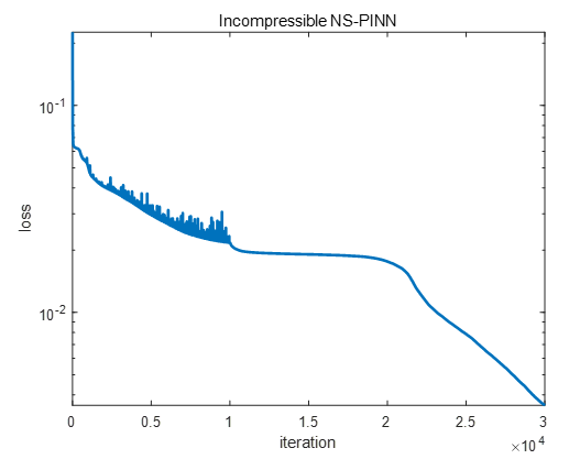
Adam 옵티마이저를 이용한 10,000번의 iteration과 바로 이어서 L-BFGS-B 옵티마이저를 이용한 20,000번의 iteration을 수행한 결과, 손실값은 다음과 같다.
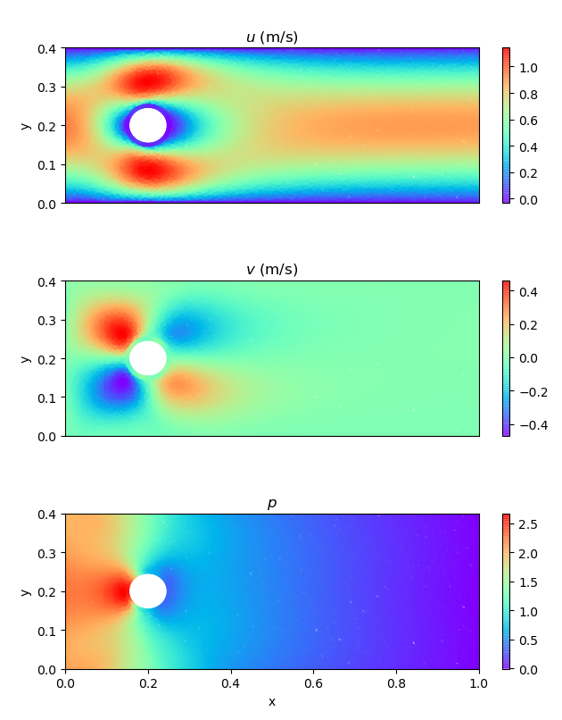
학습 결과, 실린더 주위의 유동의 속도와 압력은 다음과 같다. C. Rao의 논문 “Physics-informed deep learning for incompressible laminar flows”에 실린 Fluent 수치해 결과와 비교하면 매우 정확하다는 것을 알 수 있다.
비압축성 유동에 대한 PINN의 전체 코드는 다음과 같다.
flow_boundary_condition.py
# Setting boundary conditions
# PINN for incompressible 2-D NS equation (steady version)
# coded by St.Watermelon

import tensorflow as tf
import numpy as np


# remove collocation points inside the cylinder
def remove_pt_inside_cyl(xy_col, xc, yc, r):
    dst = np.array([((xy[0] - xc) ** 2 + (xy[1] - yc) ** 2) ** 0.5 for xy in xy_col])
    return xy_col[dst > r, :]

# define boundary condition
def func_u0(y):
    return 4.0 * y * (0.4 - y) / (0.4 ** 2)


def flow_data():
    # set number of data points
    N_b = 200    # inlet and outlet boundary
    N_w = 400    # wall boundary
    N_s = 200    # surface boundary
    N_c = 40000  # collocation points
    N_r = 10000  # additional refining points

    # set boundary
    xmin = 0.0
    xmax = 1.0
    ymin = 0.0
    ymax = 0.4
    r = 0.05
    xc = 0.2
    yc = 0.2

    # inlet boundary data, v=0
    inlet_xy = np.linspace([xmin, ymin], [xmin, ymax], N_b)
    inlet_u = func_u0(inlet_xy[:, 1]).reshape(-1,1)
    inlet_v = np.zeros((N_b,1))
    inlet_uv = np.concatenate([inlet_u, inlet_v], axis=1)

    # outlet boundary condition, p=0
    outlet_xy = np.linspace([xmax, ymin], [xmax, ymax], N_b)
    outlet_p = np.zeros((N_b, 1))

    # wall boundary condition, u=v=0
    wallup_xy = np.linspace([xmin, ymax], [xmax, ymax], N_w)
    walldn_xy = np.linspace([xmin, ymin], [xmax, ymin], N_w)
    wallup_uv = np.zeros((N_w, 2))
    walldn_uv = np.zeros((N_w, 2))

    # cylinder surface, u=v=0
    theta = np.linspace(0.0, 2 * np.pi, N_s)
    cyld_x = (r * np.cos(theta) + xc).reshape(-1, 1)
    cyld_y = (r * np.sin(theta) + yc).reshape(-1, 1)
    cyld_xy = np.concatenate([cyld_x, cyld_y], axis=1)
    cyld_uv = np.zeros((N_s, 2))

    # all boundary conditions except outlet
    xy_bnd = np.concatenate([inlet_xy, wallup_xy, walldn_xy, cyld_xy], axis=0)
    uv_bnd_sol = np.concatenate([inlet_uv, wallup_uv, walldn_uv, cyld_uv], axis=0)

    # collocation points
    x_col = np.random.uniform(xmin, xmax, [N_c, 1])
    y_col = np.random.uniform(ymin, ymax, [N_c, 1])
    xy_col = np.concatenate([x_col, y_col], axis=1)
    # refine points around cylider
    x_col_refine = np.random.uniform(xc-2*r, xc+2*r, [N_r, 1])
    y_col_refine = np.random.uniform(yc-2*r, yc+2*r, [N_r, 1])
    xy_col_refine = np.concatenate([x_col_refine, y_col_refine], axis=1)
    xy_col = np.concatenate([xy_col, xy_col_refine], axis=0)

    # remove collocation points inside the cylinder
    xy_col = remove_pt_inside_cyl(xy_col, xc=xc, yc=yc, r=r)

    # concatenation of all boundary and collocation points
    xy_col = np.concatenate([xy_col, xy_bnd, outlet_xy], axis=0)

    # convert all to tensors
    xy_col = tf.convert_to_tensor(xy_col, dtype=tf.float32)
    xy_bnd = tf.convert_to_tensor(xy_bnd, dtype=tf.float32)
    uv_bnd_sol = tf.convert_to_tensor(uv_bnd_sol, dtype=tf.float32)
    outlet_xy = tf.convert_to_tensor(outlet_xy, dtype=tf.float32)
    outlet_p = tf.convert_to_tensor(outlet_p, dtype=tf.float32)

    return xy_col, xy_bnd, uv_bnd_sol, outlet_xy, outlet_p
flow_model_lbfgs.py
# PINN for incompressible 2-D NS equation (steady version)
# coded by St.Watermelon

from flow_boundary_condition import flow_data
import tensorflow as tf
from tensorflow.keras.models import Model
from tensorflow.keras.layers import Dense
from tensorflow.keras.optimizers import Adam
import matplotlib.pyplot as plt
import numpy as np
import scipy.optimize
from time import time

class IncompressibleNet(Model):

    def __init__(self):
        super(IncompressibleNet, self).__init__()

        initializer = tf.keras.initializers.GlorotUniform
        self.h1 = Dense(50, activation='tanh', kernel_initializer=initializer)
        self.h2 = Dense(50, activation='tanh', kernel_initializer=initializer)
        self.h3 = Dense(50, activation='tanh', kernel_initializer=initializer)
        self.h4 = Dense(50, activation='tanh', kernel_initializer=initializer)
        self.h5 = Dense(50, activation='tanh', kernel_initializer=initializer)
        self.u = Dense(6, activation='linear', kernel_initializer=initializer)


    def call(self, pos):
        x = self.h1(pos)  # pos = (x, y)
        x = self.h2(x)
        x = self.h3(x)
        x = self.h4(x)
        x = self.h5(x)
        out = self.u(x)  # u,v,p,sig_xx,sig_xy,sig_yy

        u = out[:, 0:1]
        v = out[:, 1:2]
        p = out[:, 2:3]
        sig_xx = out[:, 3:4]
        sig_xy = out[:, 4:5]
        sig_yy = out[:, 5:6]
        return u, v, p, sig_xx, sig_xy, sig_yy


class NSpinn(object):

    def __init__(self):

        self.lr = 0.0005
        self.opt = Adam(self.lr)

        # density and viscosity
        self.rho = 1.0
        self.mu = 0.02

        self.flow = IncompressibleNet()
        self.flow.build(input_shape=(None, 2))

        self.train_loss_history = []
        self.iter_count = 0
        self.instant_loss = 0

    def ns_net(self, xy):
        x = xy[:, 0:1]
        y = xy[:, 1:2]

        with tf.GradientTape(persistent=True) as tape:
            tape.watch(x)
            tape.watch(y)
            xy_c = tf.concat([x,y], axis=1)
            u, v, p, sig_xx, sig_xy, sig_yy = self.flow(xy_c)
            u_x = tape.gradient(u, x)
        u_y = tape.gradient(u, y)
        v_x = tape.gradient(v, x)
        v_y = tape.gradient(v, y)
        sig_xx_x = tape.gradient(sig_xx, x)
        sig_yy_y = tape.gradient(sig_yy, y)
        sig_xy_x = tape.gradient(sig_xy, x)
        sig_xy_y = tape.gradient(sig_xy, y)
        del tape

        r_1 = self.rho * (u*u_x+v*u_y) - sig_xx_x - sig_xy_y
        r_2 = self.rho * (u*v_x+v*v_y) - sig_xy_x - sig_yy_y
        r_3 = -p + 2*self.mu*u_x - sig_xx
        r_4 = -p + 2*self.mu*v_y - sig_yy
        r_5 = self.mu*(u_y+v_x) - sig_xy
        r_6 = u_x+v_y

        return r_1, r_2, r_3, r_4, r_5, r_6


    def compute_loss(self, r_1, r_2, r_3, r_4, r_5, r_6,  \
                    u_hat, v_hat, uv_bnd_sol, p_hat, outlet_p):
        u_sol = uv_bnd_sol[:, 0:1]
        v_sol = uv_bnd_sol[:, 1:2]
        loss_bnd = tf.reduce_mean(tf.square(u_hat-u_sol)) \
                 + tf.reduce_mean(tf.square(v_hat-v_sol))
        loss_outlet = tf.reduce_mean(tf.square(p_hat-outlet_p))
        loss_col = tf.reduce_mean(tf.square(r_1)) \
                 + tf.reduce_mean(tf.square(r_2)) \
                 + tf.reduce_mean(tf.square(r_3)) \
                 + tf.reduce_mean(tf.square(r_4)) \
                 + tf.reduce_mean(tf.square(r_5)) \
                 + tf.reduce_mean(tf.square(r_6))

        return loss_bnd+loss_outlet+loss_col


    def save_weights(self, path):
        self.flow.save_weights(path + 'flow.h5')


    def load_weights(self, path):
        self.flow.load_weights(path + 'flow.h5')


    def compute_grad(self, xy_col, xy_bnd, uv_bnd_sol, outlet_xy, outlet_p):
        with tf.GradientTape() as tape:
            r_1, r_2, r_3, r_4, r_5, r_6 = self.ns_net(xy_col)
            u_hat, v_hat, _, _, _, _ = self.flow(xy_bnd)
            _, _, p_hat, _, _, _ = self.flow(outlet_xy)
            loss = self.compute_loss(r_1, r_2, r_3, r_4, r_5, r_6, \
                                     u_hat, v_hat, uv_bnd_sol, \
                                     p_hat, outlet_p)

        grads = tape.gradient(loss, self.flow.trainable_variables)

        return loss, grads


    def callback(self, arg=None):
        if self.iter_count % 10 == 0:
            print('iter=', self.iter_count, ', loss=', self.instant_loss)
            self.train_loss_history.append([self.iter_count, self.instant_loss])
        self.iter_count += 1


    def train_with_adam(self, xy_col, xy_bnd, uv_bnd_sol, outlet_xy, outlet_p, adam_num):

        @tf.function
        def learn():
            loss, grads = self.compute_grad(xy_col, xy_bnd, \
                                            uv_bnd_sol, outlet_xy, outlet_p)
            self.opt.apply_gradients(zip(grads, self.flow.trainable_variables))

            return loss

        for iter in range(int(adam_num)):

            loss = learn()

            self.instant_loss = loss.numpy()
            self.callback()


    def train_with_lbfgs(self, xy_col, xy_bnd, uv_bnd_sol, outlet_xy, outlet_p, lbfgs_num):

        def vec_weight():
            # vectorize weights
            weight_vec = []

            # Loop over all weights
            for v in self.flow.trainable_variables:
                weight_vec.extend(v.numpy().flatten())

            weight_vec = tf.convert_to_tensor(weight_vec)
            return weight_vec
        w0 = vec_weight().numpy()

        def restore_weight(weight_vec):
            # restore weight vector to model weights
            idx = 0
            for v in self.flow.trainable_variables:
                vs = v.shape

                # weight matrices
                if len(vs) == 2:
                    sw = vs[0] * vs[1]
                    updated_val = tf.reshape(weight_vec[idx:idx + sw], (vs[0], vs[1]))
                    idx += sw

                # bias vectors
                elif len(vs) == 1:
                    updated_val = weight_vec[idx:idx + vs[0]]
                    idx += vs[0]

                # assign variables (Casting necessary since scipy requires float64 type)
                v.assign(tf.cast(updated_val, dtype=tf.float32))


        def loss_grad(w):
            # update weights in model
            restore_weight(w)

            loss, grads = self.compute_grad(xy_col, xy_bnd, \
                                            uv_bnd_sol, outlet_xy, outlet_p)
            # vectorize gradients
            grad_vec = []
            for g in grads:
                grad_vec.extend(g.numpy().flatten())

            # gradient list to array
            # scipy-routines requires 64-bit floats
            loss = loss.numpy().astype(np.float64)
            self.instant_loss = loss
            grad_vec = np.array(grad_vec, dtype=np.float64)

            return loss, grad_vec

        return scipy.optimize.minimize(fun=loss_grad,
                                       x0=w0,
                                       jac=True,
                                       method='L-BFGS-B',
                                       callback=self.callback,
                                       options={'maxiter': lbfgs_num,
                                                'maxfun': 50000,
                                                'maxcor': 50,
                                                'maxls': 50,
                                                'ftol': 1.0 * np.finfo(float).eps})


    def predict(self, xy):
        u, v, p, _, _, _ = self.flow(xy)
        return u, v, p


    def train(self, adam_num, lbfgs_num):

        xy_col, xy_bnd, uv_bnd_sol, outlet_xy, outlet_p = flow_data()

        # Start timer
        t0 = time()
        self.train_with_adam(xy_col, xy_bnd, uv_bnd_sol, outlet_xy, outlet_p, adam_num)
        # Print computation time
        print('\nComputation time of adam: {} seconds'.format(time() - t0))
        t1 = time()
        self.train_with_lbfgs(xy_col, xy_bnd, uv_bnd_sol, outlet_xy, outlet_p, lbfgs_num)
        # Print computation time
        print('\nComputation time of L-BFGS-B: {} seconds'.format(time() - t1))

        self.save_weights("./save_weights/")

        np.savetxt('./save_weights/loss.txt', self.train_loss_history)
        train_loss_history = np.array(self.train_loss_history)

        plt.plot(train_loss_history[:, 0], train_loss_history[:, 1])
        plt.yscale("log")
        plt.show()


# main
def main():

    adam_num = 10001
    lbfgs_num = 20000
    agent = NSpinn()

    agent.train(adam_num, lbfgs_num)


if __name__=="__main__":
    main()
'AI 딥러닝 > DLA' 카테고리의 다른 글
| [U-Net] U-Net 구조 (0) | 2022.05.11 |
|---|---|
| [PINN] 버거스 방정식 기반 신경망 (Burgers’ Equation-Informed Neural Network) 코드 업데이트 (0) | 2022.01.11 |
| [PINN] 물리 정보 신경망 (Physics-Informed Neural Network) (0) | 2021.09.19 |
| [CNN] 컨볼루션과 상관도 (0) | 2020.09.22 |
| [CNN] 이미지 필터 설계해 보기 (0) | 2020.07.29 |


댓글