유체(fluid)나 탄성체 또는 변형체의 운동 법칙을 표현하거나 또는 여러가지 공학적인 문제를 모델링하고 해석하는데 편미분 방정식(PDE, partial differential equation)이 사용된다. 예를 들면 유체 운동의 지배 방정식인 나비어-스톡스(Navier-Stokes) 방정식을 들 수 있겠다.
편미분 방정식은 특수한 경우를 제외하고는 해석적인 해를 구할 수 없기 때문에 수치적인 방법을 사용한다. 전통적인 수치 방법은 유한차분법(FDM), 유한요소법(FEM), 또는 유한체적법(FVM)등이 있다. 이 방법들은 기본적으로 메쉬(mesh)기반으로서 계산 영역을 수많은 작은 메쉬로 분할하고 각 메쉬 포인트에서 수치해를 얻는 것이다. 이와 같은 수치적 방법은 편미분 방정식의 연구를 크게 촉진했으나 계산량이 매우 많으며 복잡한 형상에서는 적용하기 어려운 단점이 있다.
전통적인 방법 이외에 신경망을 이용하여 편미분 방정식을 수치적으로 풀기 위한 방법이 수십년 전부터 개발되어 왔는데, 이는 신경망이 임의의 정확도로 모든 연속 함수를 근사할 있는 보편적인 근사자(universal approximator)라는 배경에서 출발한 것이다.
제안된 여러 방법 중에서 최근 Raissi가 개발한 물리 정보 신경망(PINN, physics-informed neural network)이 큰 주목을 받고 있다. 왜냐하면 PINN은 신경망의 구조가 간단하고 직관적이며, 기존의 전통적인 수치방법과는 달리 메쉬가 필요없는 이른바 mesh-free 방법이라서 복잡한 형상에도 매우 효과적으로 적용할 수 있고, 비교적 빠른 시간에 정확한 PDE해를 얻을 수 있기 때문이다.
기존의 신경망이 데이터에 포함된 물리적 법칙을 고려하지 않고 데이터 중심 접근 방식에 전적으로 의존하는 데에 반해 PINN은 편미분 방정식을 충족하도록 강제하는 방식으로 편미분 방정식에 내재되어 있는 물리 정보를 신경망에 도입한다. 이를 통해 신경망 학습에 필요한 데이터를 줄일 수 있고 학습 속도를 빠르게 할 수 있는 것이다.
PINN의 구조는 아래와 같다.
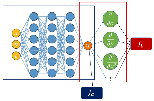
왼쪽은 데이터만 주어지는 일반적인 신경망이고, 오른쪽은 편미분 방정식을 구현한 것으로 물리 정보를 담고 있는 신경망이다. 손실함수는 왼쪽 신경망의 데이터 손실함수 \(J_d\) 와 오른쪽 신경망의 물리 정보 손실함수 \(J_p\) 로 구성된다.
데이터 손실함수 \(J_d\) 는 초기조건이나 경계조건을 만족하는 지를 평가하는 함수이고 물리 정보 손실함수 \(J_p\) 는 콜로케이션(collocation) 포인트에서 편미분 방정식을 충족하는지를 평가하는 함수이다.
PINN을 처음 제안한 Raissi의 논문에 실려 있는 버거스 방정식(Burgers' equation)을 이용하여 구체적으로 PINN을 살펴보자.
버거스 방정식과 초기조건, 경계조건은 다음과 같다.
\[ \begin{align} & u_t +uu_x -\left( \frac{0.01}{\pi} \right) u_{xx} = 0, \ \ \ \ \ x \in [-1, 1], \ \ t \in [0, 1] \\ \\ & u(x,0) = - \sin (\pi x ) \\ \\ & u(-1,t)=u(1,t)=0 \end{align} \]
여기서 \(u_t= \partial u/ \partial t\), \( u_x=∂u/∂x \), \(u_{xx}= \partial^2 u/ \partial x^2 \) 을 나타낸다.
그림 왼쪽의 데이터 신경망은 입력이 \(x\) 와 \(t\) 이고 출력이 편미분 방정식의 근사해 \(u(x,t)\) 인 완전연결 신경망으로 구현할 수 있다. \(u(x,t)\) 신경망은 6개의 hidden layer로 구성되어 있으며 각 레이어는 20개의 뉴런을 가진다. 활성함수로는 'tanh' 를 사용했다.
class Burgers(Model):

    def __init__(self):
        super(Burgers, self).__init__()

        self.h1 = Dense(20, activation='tanh')
        self.h2 = Dense(20, activation='tanh')
        self.h3 = Dense(20, activation='tanh')
        self.h4 = Dense(20, activation='tanh')
        self.h5 = Dense(20, activation='tanh')
        self.h6 = Dense(20, activation='tanh')
        self.u = Dense(1, activation='linear')


    def call(self, state):
        x = self.h1(state)
        x = self.h2(x)
        x = self.h3(x)
        x = self.h4(x)
        x = self.h5(x)
        x = self.h6(x)
        out = self.u(x)
        return out
물리정보 신경망은 \(u_t, u_x, u_{xx}\) 를 계산하는 신경망으로서 텐서플로의 자동미분 기능을 이용하여 구현할 수 있다. 물리 정보 신경망의 출력은 버거스 방정식 \(u_t+uu_x-(0.01/\pi) u_{xx}\) 이다.
많은 논문들이 Tensorflow1 기반 코드를 제공하고 있는데, 여기에서는 Tensorflow2 로 코드를 작성했다.
    def physics_net(self, xt):
        x = xt[:, 0:1]
        t = xt[:, 1:2]

        with tf.GradientTape(persistent=True) as tape:
            tape.watch(t)
            tape.watch(x)
            xt_t = tf.concat([x,t], axis=1)
            u = self.burgers(xt_t)
            u_x = tape.gradient(u, x)
        u_xx = tape.gradient(u_x, x)
        u_t = tape.gradient(u, t)
        del tape

        return u_t + u*u_x - (0.01/np.pi)*u_xx
데이터 손실함수 \(J_d\) 는 초기조건과 경계조건을 충족하도록 다음과 같이 정한다.
\[ J_d = \frac{1}{N_d} \sum_{i=1}^{N_d} \left( u (x_d^{(i) }, t_d^{(i) } ) - u^{(i) } \right)^2 \]
여기서 \(x_d^{(i) }, t_d^{(i) }, u^{(i) }\) 는 초기조건과 경계조건 데이터이다. \(N_d\) 는 데이터 갯수로서 여기서는 초기조건과 경계조건 데이터 각각 500개를 사용했다.
	# initial and boundary condition
        x_data = np.linspace(-1.0, 1.0, 500)
        t_data = np.linspace(0.0, 1.0, 500)
        xt_bnd_data = []
        tu_bnd_data = []

        for x in x_data:
            xt_bnd_data.append([x, 0])
            tu_bnd_data.append([-np.sin(np.pi * x)])

        for t in t_data:
            xt_bnd_data.append([1, t])
            tu_bnd_data.append([0])
            xt_bnd_data.append([-1, t])
            tu_bnd_data.append([0])

        xt_bnd_data = np.array(xt_bnd_data)
        tu_bnd_data = np.array(tu_bnd_data)
물리 정보 손실함수 \(J_p\) 는 콜로케이션(collocation) 포인트에서 편미분 방정식을 만족하도록 다음과 같이 정한다.
\[ J_p = \frac{1}{N_p} \sum_{i=1}^{N_p} \left( f (x_p^{(i) }, t_p^{(i) } ) \right)^2 \]
여기서
\[ f(x,t)=u_t+uu_x-\left( \frac{0.01}{\pi} \right) u_{xx} \]
이다. \(N_p\) 는 콜로케이션 포인트 갯수로서 여기서는 20,000개로 했다. 초기조건과 경계조건에서도 편미분 방정식이 성립해야 하므로 초기조건과 경계조건 데이터도 모두 콜로케이션 포인트에 포함시켰다.
        # collocation point
        t_col_data = np.random.uniform(0, 1, [20000, 1])
        x_col_data = np.random.uniform(-1, 1, [20000, 1])
        xt_col_data = np.concatenate([x_col_data, t_col_data], axis=1)
        xt_col_data = np.concatenate((xt_col_data, xt_bnd_data), axis=0)
다음 그림에서 X는 초기조건과 경계조건 데이터이고, O는 콜로케이션 데이터를 나타낸다.

총 손실함수는 \(J=J_d+J_p\) 이다.
많은 논문들이 옵티마이저로서 'L-BFGS-B' 를 사용했는데 Tensorflow2에서는 사용하기가 조금 복잡하므로 여기서는 Adam 옵티마이저를 사용했다. 3000번 의 iteration을 수행한 결과 손실값은 다음과 같다.

학습 결과, 버거스 방정식의 해는 다음과 같다. 그림은 각각 \(t=0.25, t=0.5, t=0.75\) 에서의 해를 나타낸다. 버거스 방정식의 정확한 해가 무한급수로 주어지므로 여기서는 생략했지만, Raissi의 논문과 비교하면 매우 정확하다는 것을 알 수 있다.

전체 계산 영역 \( x \in [-1,1], \ t \in [0,1] \) 에서 버거스 방정식의 해는 다음과 같다.

PINN은 편미분 방정식 연구에서 큰 잠재력을 가지고 있는 것으로 보이며, 앞으로 더욱 발전한다면 기존 Fluent나 OpenFOAM을 대체할 수 있는 신경망 기반 상업용 수치해석 솔버가 될 수도 있을 것 같다는 생각이 든다.
다음은 버거스 방정식에 대한 PINN의 전체 코드다.
# PINN for Burgers' equation
# coded by St.Watermelon

import tensorflow as tf
from tensorflow.keras.models import Model
from tensorflow.keras.layers import Dense
from tensorflow.keras.optimizers import Adam
import matplotlib.pyplot as plt
import numpy as np

class Burgers(Model):

    def __init__(self):
        super(Burgers, self).__init__()

        self.h1 = Dense(20, activation='tanh')
        self.h2 = Dense(20, activation='tanh')
        self.h3 = Dense(20, activation='tanh')
        self.h4 = Dense(20, activation='tanh')
        self.h5 = Dense(20, activation='tanh')
        self.h6 = Dense(20, activation='tanh')
        self.u = Dense(1, activation='linear')


    def call(self, state):
        x = self.h1(state)
        x = self.h2(x)
        x = self.h3(x)
        x = self.h4(x)
        x = self.h5(x)
        x = self.h6(x)
        out = self.u(x)
        return out


class Pinn(object):

    def __init__(self):

        self.lr = 0.001
        self.opt = Adam(self.lr)

        self.burgers = Burgers()
        self.burgers.build(input_shape=(None, 2))

    def physics_net(self, xt):
        x = xt[:, 0:1]
        t = xt[:, 1:2]

        with tf.GradientTape(persistent=True) as tape:
            tape.watch(t)
            tape.watch(x)
            xt_t = tf.concat([x,t], axis=1)
            u = self.burgers(xt_t)
            u_x = tape.gradient(u, x)
        u_xx = tape.gradient(u_x, x)
        u_t = tape.gradient(u, t)
        del tape

        return u_t + u*u_x - (0.01/np.pi)*u_xx


    def save_weights(self, path):
        self.burgers.save_weights(path + 'burgers.h5')


    def load_weights(self, path):
        self.burgers.load_weights(path + 'burgers.h5')


    def learn(self, xt_col, xt_bnd, tu_bnd):
        with tf.GradientTape() as tape:
            f = self.physics_net(xt_col)
            loss_col = tf.reduce_mean(tf.square(f))

            tu_bnd_hat = self.burgers(xt_bnd)
            loss_bnd = tf.reduce_mean(tf.square(tu_bnd_hat-tu_bnd))

            loss = loss_col + loss_bnd

        grads = tape.gradient(loss, self.burgers.trainable_variables)
        self.opt.apply_gradients(zip(grads, self.burgers.trainable_variables))

        return loss


    def predict(self, xt):
        tu = self.burgers(xt)
        return tu


    def train(self, max_num):

        # initial and boundary condition
        x_data = np.linspace(-1.0, 1.0, 500)
        t_data = np.linspace(0.0, 1.0, 500)
        xt_bnd_data = []
        tu_bnd_data = []

        for x in x_data:
            xt_bnd_data.append([x, 0])
            tu_bnd_data.append([-np.sin(np.pi * x)])

        for t in t_data:
            xt_bnd_data.append([1, t])
            tu_bnd_data.append([0])
            xt_bnd_data.append([-1, t])
            tu_bnd_data.append([0])

        xt_bnd_data = np.array(xt_bnd_data)
        tu_bnd_data = np.array(tu_bnd_data)

        # collocation point
        t_col_data = np.random.uniform(0, 1, [20000, 1])
        x_col_data = np.random.uniform(-1, 1, [20000, 1])
        xt_col_data = np.concatenate([x_col_data, t_col_data], axis=1)
        xt_col_data = np.concatenate((xt_col_data, xt_bnd_data), axis=0)

        train_loss_history = []

        for iter in range(int(max_num)):

            loss = self.learn(tf.convert_to_tensor(xt_col_data, dtype=tf.float32),
                       tf.convert_to_tensor(xt_bnd_data, dtype=tf.float32),
                       tf.convert_to_tensor(tu_bnd_data, dtype=tf.float32))

            train_loss_history.append([iter, loss.numpy()])

            print('iter=', iter, ', loss=', loss.numpy())

        self.save_weights("./save_weights/")

        np.savetxt('./save_weights/loss.txt', train_loss_history)
        train_loss_history = np.array(train_loss_history)

        plt.plot(train_loss_history[:, 0], train_loss_history[:, 1])
        plt.yscale("log")
        plt.show()


def main():

    max_num = 3000
    agent = Pinn()

    agent.train(max_num)


if __name__=="__main__":
    main()
'AI 딥러닝 > DLA' 카테고리의 다른 글
| [PINN] 버거스 방정식 기반 신경망 (Burgers’ Equation-Informed Neural Network) 코드 업데이트 (0) | 2022.01.11 |
|---|---|
| [PINN] 비압축성 유체 정보 기반 신경망 (Incompressible NS-Informed Neural Network) (0) | 2021.11.02 |
| [CNN] 컨볼루션과 상관도 (0) | 2020.09.22 |
| [CNN] 이미지 필터 설계해 보기 (0) | 2020.07.29 |
| [CNN] 2D 컨볼루션 계산하기 (0) | 2020.07.29 |


댓글