섭동력을 받는 램버트 문제의 보정 해

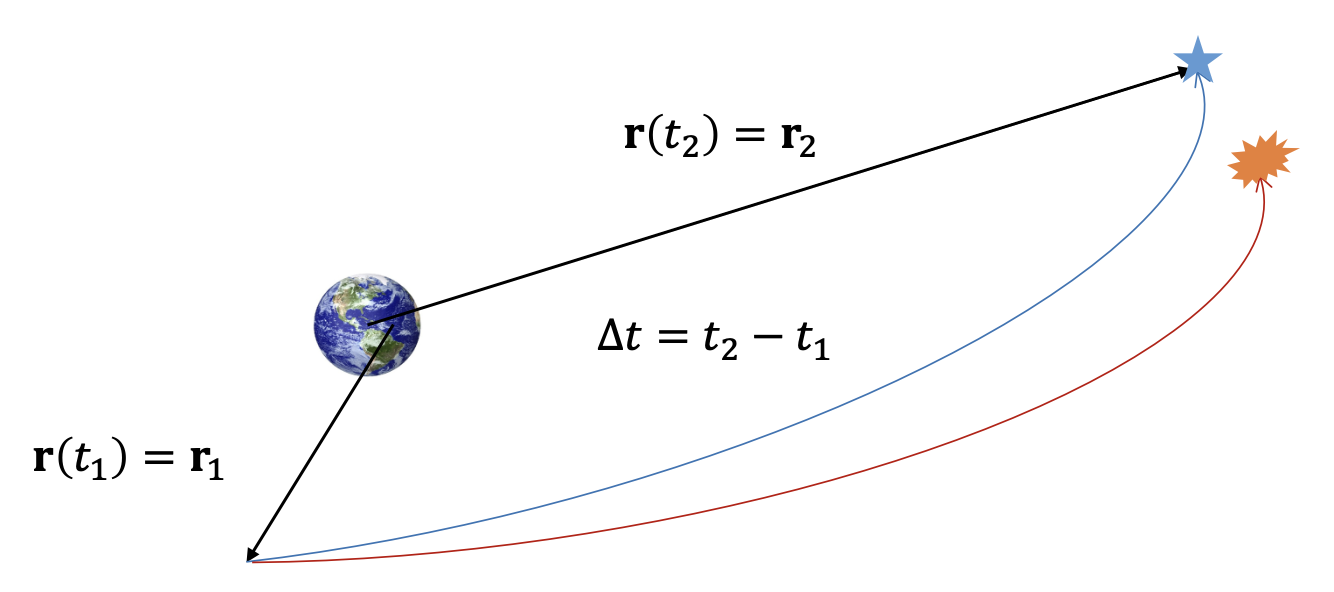
램버트 문제의 해(https://pasus.tistory.com/316)는 두 위치 ${\mathbf{r}}_1$ 과 ${\mathbf{r}}_2$ 사이를 비행하는 데 걸리는 시간 $\mathrm{\Delta }t$ 가 주어졌을 때, 두 위치를 연결하는 이체문제 (two-body problem) 궤적(trajectory)을 계산한다. 하지만 램버트 문제에서 고려하지 않았던 섭동력(perturbation)으로 인하여 궤적이 목표로 한 위치 ${\mathbf{r}}_2$ 에 도달하지 못할 때는 어떻게 해야 할까.

 

 

일반적인 섭동력 (J2 섭동력, 태양복사압력, 항력, 달 또는 태양 등의 제3의 중력 등)의 경우 이러한 오차 거리(miss distance)가 크지 않기 때문에, 출발 위치 ${\mathbf{r}}_1$ 에서 램버트 솔버가 산출한 속도벡터 ${\mathbf{v}}_1$ 을 보정하여 최종 위치 ${\mathbf{r}}_2$ 에서 오차 거리를 줄일 수 있다. 이와 같은 방법을 슈팅방법(shooting method)이라고 한다(https://pasus.tistory.com/276).

슈팅방법은 기본적으로 경계값 문제를 초기값 문제로 바꾸어 해를 구하는 방법으로서, 초기값으로부터 산출된 최종값과 목표값 간의 차이를 이용하여 원래 초기값을 수정한다.

최종 위치 오차 $\mathrm{\Delta }{\mathbf{r}}_2$ 는 출발 위치에서의 속도벡터 섭동 $\mathrm{\Delta }{\mathbf{v}}_1$ 을 이용하여 다음과 같이 근사적으로 표현할 수 있다.

 

$$\begin{array}{}\text{(1)}& \mathrm{\Delta }{\mathbf{r}}_2=\frac{d{\mathbf{r}}_2}{d{\mathbf{v}}_1}\mathrm{\Delta }{\mathbf{v}}_1\end{array}$$

 

여기서 미분 $\frac{d{\mathbf{r}}_2}{d{\mathbf{v}}_1}$ 는 자코비안(Jacobian)으로서 $3\times 3$ 행렬인데, 출발 위치에서의 초기 속도변화에 대한 최종 위치의 변화를 나타내므로 '민감도' 행렬이라고도 한다.

식 (1)에 의하면 최종 위치벡터 오차에 대한 초기 속도벡터 오차 $\mathrm{\Delta }{\mathbf{v}}_1$ 은 다음과 같이 추정할 수 있다.

 

$$\begin{array}{}\text{(2)}& \mathrm{\Delta }{\mathbf{v}}_1={\left(\frac{d{\mathbf{r}}_2}{d{\mathbf{v}}_1}\right)}^{-1}\mathrm{\Delta }{\mathbf{r}}_2\end{array}$$

 

추정된 속도벡터 오차를 속도벡터 ${\mathbf{v}}_1$ 에서 빼주면 ${\mathbf{v}}_1$ 을 새로운 값으로 업데이트할 수 있다.

 

$$\begin{array}{r}\text{(3)}& {\mathbf{v}}_1& \leftarrow {\mathbf{v}}_1-\mathrm{\Delta }{\mathbf{v}}_1\\ & ={\mathbf{v}}_1-{\left(\frac{d{\mathbf{r}}_2}{d{\mathbf{v}}_1}\right)}^{-1}\mathrm{\Delta }{\mathbf{r}}_2\end{array}$$

 

식 (2)의 자코비안 또는 민감도 행렬 $\frac{d{\mathbf{r}}_2}{d{\mathbf{v}}_1}$ 의 구성 성분을 쓰면 다음과 같다.

 

$$\begin{array}{}\text{(5)}& \frac{d{\mathbf{r}}_2}{d{\mathbf{v}}_1}=\mathcal{J}=\left[\begin{array}{ccc}\frac{\partial x_2}{\partial u_1}& \frac{\partial x_2}{\partial v_1}& \frac{\partial x_2}{\partial w_1}\\ \frac{\partial y_2}{\partial u_1}& \frac{\partial y_2}{\partial v_1}& \frac{\partial y_2}{\partial w_1}\\ \frac{\partial z_2}{\partial u_1}& \frac{\partial z_2}{\partial v_1}& \frac{\partial z_2}{\partial w_1}\end{array}\right]\end{array}$$

 

여기서 ${\mathbf{r}}_2={\left[\begin{array}{ccc}{x}_2& y_2& z_2\end{array}\right]}^T$, ${\mathbf{v}}_1={\left[\begin{array}{ccc}{u}_1& v_1& w_1\end{array}\right]}^T$ 로서 각 벡터를 ECI 좌표계로 표현한 것이다.

이제 J2 섭동력 하에서도 궤적이 시간 $\mathrm{\Delta }t$ 후에 목표 위치 ${\mathbf{r}}_2$ 로 정확히 도달할 수 있도록, 램버트가 산출한 초기 속도벡터 ${\mathbf{v}}_1$ 을 슈팅방법을 이용하여 보정해 보도록 하겠다.

J2 섭동력을 포함한 램버트 문제는 다음과 같다.

 

$$\begin{array}{r}\text{(5)}& & \frac{d^2\mathbf{r}}{d{t}^2}+\frac{\mu }{r^3}\mathbf{r}={\mathbf{a}}_p\\ & {\mathbf{a}}_p=\frac{3}{2}{J}_2\frac{\mu }{r^5}{R}_e^2\left[\begin{array}{c}x(5{\left(\frac{z}{r}\right)}^2-1)\\ y(5{\left(\frac{z}{r}\right)}^2-1)\\ z(5{\left(\frac{z}{r}\right)}^2-3)\end{array}\right]\\ \\ & \mathbf{r}(t_1)={\mathbf{r}}_1,\mathbf{r}(t_2)={\mathbf{r}}_2,\mathrm{\Delta }t=t_2-t_1\end{array}$$

 

여기서 $\mathbf{r}={\left[\begin{array}{ccc}x& y& z\end{array}\right]}^T$, $r=|\mathbf{r}|$, $J_2=0.0010826269$ 이며 ${\mathbf{a}}_p$ 는 J2 섭동 가속도이다.

식 (4)에 의하면 자코비안 $\mathcal{J}$ 는 유한 차분을 사용하여 한 번에 한 열씩 수치적으로 계산할 수 있다. 방법은 다음과 같다.

$\mathcal{J}$ 의 첫번째 열을 계산하기 위하여 ${\mathbf{v}}_1$ 의 첫번째 성분에만 $+\mathrm{\Delta }$ 만큼의 조그마한 (예를 들면 $0.01km/s$) 섭동을 준다.

 

$$\begin{array}{}\text{(6)}& {\mathbf{v}}_1^{+}={\mathbf{v}}_1+\left[\begin{array}{c}+\mathrm{\Delta }\\ 0\\ 0\end{array}\right]\end{array}$$

 

그리고 ${\mathbf{r}}_1$ 과 ${\mathbf{v}}_1^{+}$ 을 초기 조건으로 삼아 식 (5)를 수치적분하여 시간 $\mathrm{\Delta }t$ 후의 위치벡터 ${\mathbf{r}}_2^{+}$ 를 계산한다. 이 단계를 슈팅 단계라고 한다.

그런 후 이번에는 ${\mathbf{v}}_1$ 의 첫번째 성분에 반대 방향으로 $-\mathrm{\Delta }$ 만큼의 섭동을 준다.

 

$$\begin{array}{}\text{(7)}& {\mathbf{v}}_1^{+}={\mathbf{v}}_1+\left[\begin{array}{c}-\mathrm{\Delta }\\ 0\\ 0\end{array}\right]\end{array}$$

 

마찬가지로 ${\mathbf{r}}_1$ 과 ${\mathbf{v}}_1^{-}$ 을 초기 조건으로 삼아 식 (4)를 수치적분하여 시간 $\mathrm{\Delta }t$ 후의 위치벡터 ${\mathbf{r}}_2^{-}$ 를 계산한다. 그러면 자코비안 $\mathcal{j}$ 의 첫번째 열을 다음과 같이 계산할 수 있다.

 

$$\begin{array}{}\text{(8)}& {\mathcal{J}}_1=\frac{{\mathbf{r}}_2^{+}-{\mathbf{r}}_2^{-}}{2\mathrm{\Delta }}\end{array}$$

 

동일한 방법으로 ${\mathbf{v}}_1$ 의 두번째 성분과 세번째 성분에만 각각 동일한 섭동을 주어서 자코비안 $\mathcal{J}$ 의 두번째 열과 세번째 열을 계산하면 자코비안 $\mathcal{J}$ 의 전체 행렬을 구할 수 있다.

 

 

자코비안을 구한 후에는 식 (3)으로 초기 속도벡터를 보정하면 된다. 그리고 다시 새로운 속도벡터를 이용하여 자코비안을 다시 계산하고 속도벡터를 보정하는 프로세스를 오차 거리가 일정 수준 이하로 작아질 때 까지 계속 반복한다.

 

 

수치 예를 들어보자. 램버트 문제의 경계조건은 다음과 같다.

 

$$\begin{array}{r}\text{(9)}& & \mathbf{r}(t_1)={\mathbf{r}}_1={\left[\begin{array}{ccc}5,000& 10,000& 2,100\end{array}\right]}^{T}km\\ & \mathbf{r}(t_2)={\mathbf{r}}_2={\left[\begin{array}{ccc}-14,600& 2,500& 7,000\end{array}\right]}^{T}km\\ \\ & \mathrm{\Delta }t=t_2-t_1=3,600sec(1hr)\end{array}$$

 

위 문제를 범용변수 기반 램버트 알고리즘(https://pasus.tistory.com/316)으로 푼 초기 속도는 다음과 같다.

 

$$\begin{array}{}\text{(10)}& \mathbf{v}(t_1)={\mathbf{v}}_1=\left[\begin{array}{c}-5.992494639666394\\ 1.925363415280893\\ 3.245636528490488\end{array}\right]km/s\end{array}$$

 

식 (5)에서 ${\mathbf{a}}_p=0$ (no J2) 으로 하고 ${\mathbf{r}}_1$ 과 ${\mathbf{v}}_1$ 을 초기 조건으로 하여 최종 위치벡터를 계산하고 오차 거리를 구하면 $5.954239\times {10}^{-9}m$ 로서 램버트 솔버가 매우 정확한 해를 구한 것을 알 수 있다. 하지만 J2를 고려했을 때, 동일한 초기 조건으로 최종 위치벡터를 계산하고 오차 거리를 구하면 $538.5933m$ 로서 오차 거리가 상당히 커진 것을 볼 수 있다.

이 오차 거리를 감소시키기 위하여 초기 속도벡터를 슈팅 방법으로 보정하면 결과는 다음과 같다. 우선 3회의 반복횟수 만에 초기 속도벡터가 다음 값으로 수정되었다.

 

$$\begin{array}{}\text{(11)}& {\mathbf{v}}_{1_{corrected}}=\left[\begin{array}{c}-5.992359526670324\\ 1.924215530723804\\ 3.246086959795341\end{array}\right]km/s\end{array}$$

 

보정된 속도와 원래 속도의 크기 차이는 $0.1240477m/s$ 에 불과할 만큼 매우 작다. 하지만 이러한 속도 차이가 상당한 크기의 오차 거리를 유발한 것이다.

이제 보정된 속도벡터를 초기값으로 하여 최종 위치벡터를 계산하고 오차 거리를 구하면 $2.746990\times {10}^{-9}m$ 로서 슈팅 방법으로 수행한 보정이 매우 정확하다는 것을 알 수 있다.

다음은 자코비안 행렬 (또는 민감도 행렬)을 계산하는 알고리즘을 매트랩 코드로 구현한 것이다.

 

jacobian_shooting.m

 

function J = jacobian_shooting(odefun, y0ini, tof, dv)

% J = jacobian_shooting(odefun, y0ini, tof, dv)
%        given odefun, y0in, tof, dv
%        compute 3x3 Jacobian for shooting method
%       
% Input  odefun: ODE function
%        y0ini: initial position and velocity vector in km, km/s
%             = [x y z vx vy vz]'
%        tof: time of flight in sec
%        dv: small velocity amoint used for finite differences in km/s
% Output J: Jacobian
%
% all in inertial frame (ECI)
%
% coded by st.watermelon

J = zeros(3, 3);

tspan = [0:tof/100:tof]';
OPTIONS = odeset('RelTol',3e-14,'AbsTol',1e-15);

% finite differences with +/- vx
y0 = y0ini + [0 0 0 +dv 0 0]';
[t,y] = ode113(odefun, tspan, y0, OPTIONS);
rplus = y(end,1:3)';
y0 = y0ini + [0 0 0 -dv 0 0]';
[t,y] = ode113(odefun, tspan, y0, OPTIONS);
rminus = y(end,1:3)';
J(:, 1) = (rplus-rminus)/(2*dv);

% finite differences with +/- vy
y0 = y0ini + [0 0 0 0 +dv 0]';
[t,y] = ode113(odefun, tspan, y0, OPTIONS);
rplus = y(end,1:3)';
y0 = y0ini + [0 0 0 0 -dv 0]';
[t,y] = ode113(odefun, tspan, y0, OPTIONS);
rminus = y(end,1:3)';
J(:, 2) = (rplus-rminus)/(2*dv);

% finite differences with +/- vz
y0 = y0ini + [0 0 0 0 0 +dv]';
[t,y] = ode113(odefun, tspan, y0, OPTIONS);
rplus = y(end,1:3)';
y0 = y0ini + [0 0 0 0 0 -dv]';
[t,y] = ode113(odefun, tspan, y0, OPTIONS);
rminus = y(end,1:3)';
J(:, 3) = (rplus-rminus)/(2*dv);

 

다음은 식 (5)의 운동 방정식을 구현한 코드다.

 

orbitbody_J2.m

 

function ydot=orbitbody_J2(t,y)

% two-body orbital equation with J2
% coded by st.watermelon

mu=398600;
Rearth=6378;
J2=1.0826269e-3;

r=y(1:3);
v=y(4:6);

normr=norm(r);
rhat=r/normr;

acc=-(mu/(normr*normr))*rhat;

% J2
tmp = 5*r(3)^2/normr^2;
acc=acc + 3/2*J2*mu/normr^5*Rearth^2* ...
          [r(1)*(tmp-1); r(2)*tmp-1; r(3)*(tmp-1)];

%acc=acc - (mu*J2*Rearth*Rearth/2)* ...
%    ((6*z/(normr^5))*khat+((3/(normr^4))-(15*z*z/(normr^6)))*rhat);
ydot=zeros(6,1);
ydot(1:3)=v;
ydot(4:6)=acc;

 

다음은 수치 예제를 실행한 파일이다.

 

orbit_simul.m

 

% 
% J2-perturbed Lambert correction with shooting method
% coded by st.watermelon

clear all


% data
r1=[5000 10000  2100]';
r2=[-14600  2500  7000]';
tof=60*60; % 1 hour

OPTIONS = odeset('RelTol',3e-14,'AbsTol',1e-15);

% 1. Lambert solution
[v1, v2] = lambert(r1, r2, tof);

% 2. check solution accuracy  
y0=[r1;v1];
[t,y]=ode113(@orbitbody, [0:60:tof]',y0,OPTIONS); 

r2_computed = y(end,1:3)';
err_is = r2_computed-r2;

fprintf('Lambert solver accuracy \n');
fprintf('final error distance = %e m \n\n', norm(err_is)*100);


% 3. check again with J2 perturbation
y0=[r1;v1];
[t,yJ2]=ode113(@orbitbody_J2, [0:60:tof]',y0,OPTIONS);

r2_J2computed = yJ2(end,1:3)';
errJ2_is = r2_J2computed-r2;

fprintf('J2-perturbed Lambert solver accuracy \n');
fprintf('final error distance = %e m \n\n', norm(errJ2_is)*100);

% 4. correction with shooting method
v1_J2 = v1;
for iter=1:10
    y0=[r1;v1_J2];
    [t,y]=ode113(@orbitbody_J2, [0:60:tof]',y0,OPTIONS);
    J = jacobian_shooting(@orbitbody_J2, [r1; v1_J2], tof, 0.01);
    correc = inv(J)*(y(end,1:3)'-r2);
    v1_J2 = v1_J2 - correc;
    if norm(correc)<1e-8
        break
    end
end
v1_J2
fprintf('shooting iteration = %d \n', iter);
fprintf('initial velocity differences = %e m/s \n\n', norm(v1-v1_J2)*100);


% 5. check corrected accuracy
y0=[r1;v1_J2];
[t,yJ2_c]=ode113(@orbitbody_J2, [0:60:tof]',y0,OPTIONS);

r2_J2c = yJ2_c(end,1:3)';
errJ2c_is = r2_J2c-r2;

fprintf('corrected solution accuracy \n');
fprintf('final error distance = %e m \n', norm(errJ2c_is)*100);