Ascher의 책 'Computer Methods for Ordinary Dierential Equations and Dierential-Algebraic Equations' 에 나와 있는 예제를 다중 슈팅방법(multiple shooting method)을 이용하여 풀어보고자 한다.
미분방정식은 다음과 같다.
\[ \begin{align} \dot{\mathbf{x}} = \begin{bmatrix} 0 & 1 & 0 \\ 0 & 0 & 1 \\ -2 \lambda^3 & \lambda^2 & 2 \lambda \end{bmatrix} \mathbf{x}+ \begin{bmatrix} 0 \\ 0 \\ q(t) \end{bmatrix} \tag{1} \end{align} \]
여기서 \(\mathbf{x}=[ x_1 \ \ x_2 \ \ x_3 ]^T\) 이며 \(q(t)\) 는 다음과 같다.
\[ \begin{align} q(t)=2 \lambda^3 \cos \pi t+ \lambda^2 \pi \sin \pi t+ 2 \lambda \pi^2 \cos \pi t+ \pi^3 \sin \pi t \tag{2} \end{align} \]
식 (1)에 다음과 같은 경계조건이 주어졌을 때
\[ \begin{align} x_1 (0) &= \beta_1 = \frac{1}{2+ e^{-\lambda} } (e^{-\lambda}+e^{-2 \lambda}+1)+1 \tag{3} \\ \\ x_1 (1) &= 0 \\ \\ x_2 (0) &= \beta_2 = \frac{\lambda}{2+e^{-\lambda} } (e^{-\lambda}+2e^{-2\lambda}-1) \end{align} \]
정답 해는 다음과 같다.
\[ \begin{align} x_1 (t)= \frac{1}{2+e^{-\lambda} } (e^{\lambda(t-1)} +e^{2 \lambda (t-1)} +e^{-\lambda t} )+ \cos \pi t \tag{4} \end{align} \]
문제는 경계조건을 만족하도록 시간 \(t=0\) 에서 \(x_3 (t)\) 의 초기값 \(x_3 (0)\) 을 구하는 것이다.
여기서 재미있는 점은 식 (1)에서 \(\lambda =1\) 일 때는 초기값의 작은 변화에 대해서 매우 안정적인 반면 \(\lambda=20\) 이상에서는 매우 불안정해진다는 것이다. 따라서 \(\lambda =1\) 일 때는 단일 또는 다중 슈팅방법 모두 잘 작동하지만, \(\lambda=20\) 에서는 단일 슈팅방법은 작동하지 않고 다중 슈팅방법만 작동한다.
먼저 단일 슈팅방법을 적용하기 위하여 이전 게시글 (https://pasus.tistory.com/331)의 알고리즘을 다시 써보자.
\[ \begin{align} & \mathbf{h}( \mathbf{c})= \mathbf{g}(\mathbf{c}, \mathbf{x}(t_f; \mathbf{c}))=0 \tag{5} \\ \\ & \mathbf{c}^{(i+1)}= \mathbf{c}^{(i)}- \left( \frac{ d \mathbf{h}}{ d \mathbf{c}} \right)^{-1}_{\mathbf{c}^{(i)} } \mathbf{h}( \mathbf{c}^{(i) } ), \ \ \ \ i=1, 2, ... \\ \\ & \left( \frac{ d \mathbf{h}}{ d \mathbf{c}} \right)_{\mathbf{c}^{(i)} } = \left( \frac{ d \mathbf{g}}{ d \mathbf{c}} \right)_{\mathbf{c}^{(i)} } \end{align} \]
본 예제의 구속조건은 다음과 같이 쓸 수 있다.
\[ \begin{align} \mathbf{h}(\mathbf{c})= \mathbf{g}( \mathbf{c}, \mathbf{x}(t_f; \mathbf{c}))= \begin{bmatrix} c_1-\beta_1 \\ c_2-\beta_2 \\ x_1 (1; c_1, c_2, c_3) \end{bmatrix} =0 \tag{6} \end{align} \]
여기서 초기값 \(x_1 (0)\) 와 \(x_2 (0)\) 는 각각 \(\beta_1\) 과 \(\beta_2\) 로 각각 정해졌으므로 초기값 벡터 \(\mathbf{c}\) 에서 미지수는 \(c_3\) 다. 식 (6)을 이용하여 자코비안 \( \left( \frac{d \mathbf{g}}{d \mathbf{c}} \right)_{\mathbf{c}^{(i)}} \) 을 계산하면 다음과 같다.
\[ \begin{align} \left( \frac{d \mathbf{g}}{d \mathbf{c}} \right)_{\mathbf{c}^{(i)}} = \begin{bmatrix} 1 & 0 & 0 \\ 0 & 1 & 0 \\ \frac{ \partial x_1^{(i)} (1) }{ \partial c_1^{(i)} } & \frac{ \partial x_1^{(i)} (1) }{ \partial c_2^{(i)} } & \frac{ \partial x_1^{(i)} (1) }{ \partial c_3^{(i)} } \end{bmatrix} \tag{7} \end{align} \]
식 (7)을 식 (5)의 업데이트 식에 대입하면 다음과 같다.
\[ \begin{align} & c_1^{(i+1)}-c_1^{(i) }= -(c_1^{(i) }- \beta_1 ) \ \ \to \ \ c_1^{(i+1)}= \beta_1 \tag{8} \\ \\ & c_2^{(i+1)}-c_2^{(i)}= -(c_2^{(i)}-\beta_2 ) \ \ \to \ \ c_2^{(i+1)}= \beta_2 \end{align} \]
식 (8)과 식 (6)의 구속조건을 고려하면 \(c_1\) 과 \(c_2\) 의 업데이트 식은 다음과 같다.
\[ \begin{align} & c_1^{(1)}= \beta_1 \ \ \to \ \ c_1^{(i+1)}=c_1^{(i)}= \beta_1 \tag{9} \\ \\ & c_2^{(1)}= \beta_2 \ \ \to \ \ c_2^{(i+1)}-c_2^{(i)}= \beta_2 \end{align} \]
\(c_3\) 의 업데이트 식은 식 (9)를 고려하여 식 (7)과 (5)로부터 구할 수 있다.
\[ \begin{align} & \frac{ \partial x_1^{(i)} (1)}{ \partial c_3^{(i)} } (c_3^{(i+1)}-c_3^{(i)} ) = - x_1^{(i)} (1) \tag{10} \\ \\ & \to \ \ c_3^{(i+1)}=c_3^{(i)}- \left( \frac{ \partial x_1^{(i)} (1)}{ \partial c_3^{(i)} } \right)^{-1} x_1^{(i)} (1), \ \ \ \ i=1, 2, ... \end{align} \]
이 부분을 매트랩 코드로 구현하면 다음과 같다.
% single shooting -------------------
x03comp = 0;
for iter=1:10
    x0comp=[x0(1);x0(2);x03comp];
    [ts,xs]=ode113(@(t,x) testfun(t,x,lam), tspan_f, x0comp, OPTIONS);
    J = single_shooting(@testfun, lam, x0comp, 0.001, OPTIONS, tspan_f);
    correc = xs(end,1)/J;
    x03comp = x03comp - correc;
    if norm(correc)<1e-12
        break
    end
end

% single shooting Jacobian
function J = single_shooting(testfun, lam, x0ini, dx3, OPTIONS, tspan)

% finite differences with +/-
x0 = x0ini + [0 0 +dx3]';
[t, x] = ode113(@(t,x) testfun(t,x,lam), tspan, x0, OPTIONS);
x1plus = x(end,1)';

x0 = x0ini + [0 0 -dx3]';
[t, x] = ode113(@(t,x) testfun(t,x,lam), tspan, x0, OPTIONS);
x1minus = x(end,1)';
J = (x1plus-x1minus)/(2*dx3);

end
이번에는 다중 슈팅방법을 적용하기 위하여 마찬가지로 이전 게시글 (https://pasus.tistory.com/331)의 알고리즘을 다시 써보자.
\[ \begin{align} & \mathbf{g}( \mathbf{c}_0 , \mathbf{x}_N (t_f; \mathbf{c}_{N-1} ))=0 \tag{11} \\ \\ & \mathbf{h}(\mathbf{c})= \begin{bmatrix} \mathbf{x}_1 (t_1; \mathbf{c}_0 )- \mathbf{c}_1 \\ \mathbf{x}_2 (t_2; \mathbf{c}_1 )- \mathbf{c}_2 \\ ⋮ \\ \mathbf{x}_{N-1} (t_{N-1}; \mathbf{c}_{N-2} )- \mathbf{c}_{N-1} \\ \mathbf{g}(\mathbf{c}_0, \mathbf{x}_N (t_N; \mathbf{c}_{N-1} )) \end{bmatrix} =0 \\ \\ & \mathbf{c}^{(i+1)}= \mathbf{c}^{(i)}- \left( \frac{d \mathbf{h}}{d \mathbf{c}} \right)_{\mathbf{c}^{(i)} }^{-1} \mathbf{h}( \mathbf{c}^{(i) } ), \ \ \ \ i=1, 2, ... \end{align} \]
계산상 편의를 위해서 여기서는 노드수를 \(N=3\) 으로 정했다.

본 예제의 구속조건은 다음과 같이 쓸 수 있다.
\[ \begin{align} \mathbf{h}(\mathbf{c})= \begin{bmatrix} \mathbf{x}_1 (t_1; \mathbf{c}_0 )- \mathbf{c}_1 \\ \mathbf{x}_2 (t_2; \mathbf{c}_1 )- \mathbf{c}_2 \\ \mathbf{g}(\mathbf{c}_0, \mathbf{x}_3 (t_f; \mathbf{c}_2 )) \end{bmatrix} =0 \tag{12} \end{align} \]
여기서 미지수와 경계조건은 다음과 같다.
\[ \begin{align} \mathbf{c}= \begin{bmatrix} \mathbf{c}_0 \\ \mathbf{c}_1 \\ \mathbf{c}_2 \end{bmatrix}, \ \ \ \ \mathbf{g}(\mathbf{c}_0, \mathbf{x}_3 (t_f; \mathbf{c}_2 )) = \begin{bmatrix} c_{01}-\beta_1 \\ c_{02}-\beta_2 \\ x_{31} (1; \mathbf{c}_2 ) \end{bmatrix}=0 \tag{13} \end{align} \]
식 (12)와 (13)을 이용하여 자코비안 \( \left( \frac{d \mathbf{h}}{d \mathbf{c}} \right)_{\mathbf{c}^{(i)} } \) 을 계산하면 다음과 같다.
\[ \begin{align} \left( \frac{d \mathbf{h}}{d \mathbf{c}} \right)_{\mathbf{c}^{(i)} }= \begin{bmatrix} \frac{ \partial \mathbf{x}_1^{(i)} (t_1) }{\partial \mathbf{c}_0^{(i)} } & -I & 0 \\ 0 & \frac{ \partial \mathbf{x}_2^{(i)} (t_2) }{\partial \mathbf{c}_1^{(i)} } & -I \\ \frac{ \partial \mathbf{g}^{(i)} }{\partial \mathbf{c}_0^{(i)} } & 0 & \frac{ \partial \mathbf{g}^{(i)} }{\partial \mathbf{c}_2^{(i)} } \end{bmatrix} \tag{14} \end{align} \]
여기서 자코비안 \( \frac{ \partial \mathbf{g}^{(i)} }{\partial \mathbf{c}_0^{(i)} } \) 와 \( \frac{ \partial \mathbf{g}^{(i)} }{\partial \mathbf{c}_2^{(i)} } \) 는 각각 다음과 같다.
\[ \begin{align} & \frac{ \partial \mathbf{g}^{(i)} }{\partial \mathbf{c}_0^{(i)} } =\begin{bmatrix} 1 & 0 & 0 \\ 0 & 1 & 0 \\ 0 & 0 & 0 \end{bmatrix} \tag{15} \\ \\ & \frac{ \partial \mathbf{g}^{(i)} }{\partial \mathbf{c}_2^{(i)} } = \begin{bmatrix} 0 & 0 & 0 \\ 0 & 0 & 0 \\ \frac{ \partial x_{31}^{(i)} (1)}{\partial c_{21}^{(i)} } & \frac{ \partial x_{31}^{(i)} (1)}{\partial c_{22}^{(i)} } & \frac{ \partial x_{31}^{(i)} (1)}{\partial c_{23}^{(i)} } \end{bmatrix} \end{align} \]
식 (14)의 자코비안은 \(9 \times 9\) 행렬이므로 역행렬을 쉽게 계산할 수 있다. 이제 식 (11)의 업데이트 식으로 \(\mathbf{c}\) 를 업데이트 하면 된다. 이 부분을 매트랩 코드로 구현하면 다음과 같다.
% multiple shooting ---------------------------
% initial guess for three nodes
c0 = [x0(1); x0(2); 0];
c1 = zeros(3,1);
c2 = zeros(3,1);
cc = {c0, c1, c2};

% time at each node
t1 = 0.3; t2 = 0.7;

tspan0 = linspace(0, t1, floor(dt/3))';
tspan1 = linspace(t1, t2, floor(dt/3))';
tspan2 = linspace(t2, tf, floor(dt/3))';
tspan = {tspan0, tspan1, tspan2};

J = {}; % Jacobian
x_node = {};

%
for iter=1:10

    for j = 1:3 % for each node
        [tm,xm]=ode113(@(t,x) testfun(t,x,lam), tspan{j}, cc{j}, OPTIONS);
        J{j} = multi_shooting(@testfun, lam, cc{j}, 0.001, OPTIONS, tspan{j});
        x_node{j} = xm(end, :)';
    end
    Jlast = J{3}(1,:);

   % dgdc
    gc = [cc{1}(1)- x0(1)
          cc{1}(2)- x0(2)
          x_node{3}(1)];

    dgdc0 = [1 0 0; 0 1 0; 0 0 0];
    dgdc2 = [0 0 0; 0 0 0; Jlast];

    % dhdc
    hc = [x_node{1} - cc{2}
          x_node{2} - cc{3}
          gc ];

    dhdc = [J{1} -eye(3) zeros(3,3)
            zeros(3,3) J{2} -eye(3)
            dgdc0 zeros(3,3) dgdc2 ];

    % update
    correc = inv(dhdc)*hc;
    update = [cc{1}; cc{2}; cc{3}] - correc;
    for j = 1:3
        cc{j} = update(3*(j-1)+1:3*j);
    end

    if norm(correc)<1e-12
        break
    end

end

%%
% multiple shooting Jacobian
function J = multi_shooting(testfun, lam, x0ini, dx, OPTIONS, tspan)

J = zeros(3, 3);

% finite differences with +/- x1
x0 = x0ini + [dx 0 0]';
[t, x] = ode113(@(t,x) testfun(t,x,lam), tspan, x0, OPTIONS);
rplus = x(end,1:3)';

x0 = x0ini + [-dx 0 0]';
[t, x] = ode113(@(t,x) testfun(t,x,lam), tspan, x0, OPTIONS);
rminus = x(end,1:3)';
J(:,1) = (rplus-rminus)/(2*dx);

% finite differences with +/- x2
x0 = x0ini + [0 dx 0]';
[t, x] = ode113(@(t,x) testfun(t,x,lam), tspan, x0, OPTIONS);
rplus = x(end,1:3)';

x0 = x0ini + [0 -dx 0]';
[t, x] = ode113(@(t,x) testfun(t,x,lam), tspan, x0, OPTIONS);
rminus = x(end,1:3)';
J(:,2) = (rplus-rminus)/(2*dx);

% finite differences with +/- x3
x0 = x0ini + [0 0 dx]';
[t, x] = ode113(@(t,x) testfun(t,x,lam), tspan, x0, OPTIONS);
rplus = x(end,1:3)';

x0 = x0ini + [0 0 -dx]';
[t, x] = ode113(@(t,x) testfun(t,x,lam), tspan, x0, OPTIONS);
rminus = x(end,1:3)';
J(:,3) = (rplus-rminus)/(2*dx);

end
다음은 \(\lambda=1\) 일 때 경계값 문제를 단일 및 다중 슈팅방법으로 푼 결과를 그림으로 나타낸 것이다.

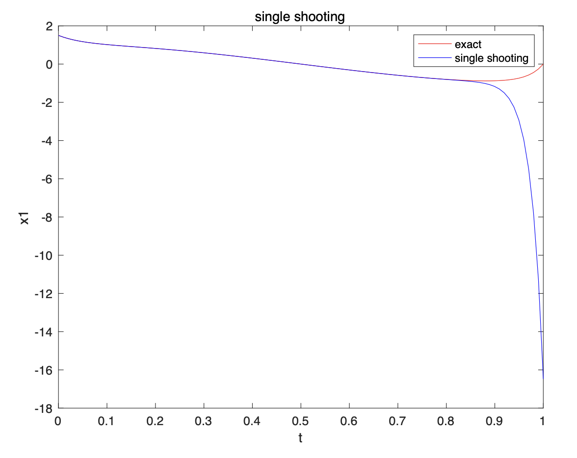
다음 그림은 \(\lambda=20\) 일 때 경계값 문제를 단일 슈팅방법으로 푼 것이다. \(x_3 (0)\) 의 값을 계산하는 데 실패했으며 큰 값으로 발산함을 알 수 있다.
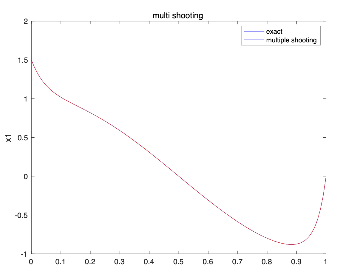
이번에는 동일한 문제를 다중 슈팅방법으로 푼 그림이다. \(\lambda=20\) 일 때의 경계값 문제를 성공적으로 푼 것을 확인할 수 있다.
다음은 본 예제에서 사용한 다중 슈팅방법의 전체 매트랩 코드다.
% Single and Multiple shooting methods
% example in Ascher's book
% coded by st.watermelon


% setting
tf = 1; dt = 100;
tx = linspace(0, tf, dt)';

lam = 1; % 20

tspan_f = linspace(0, tf, dt)';
OPTIONS = odeset('RelTol',1e-13,'AbsTol',1e-13);

% exact solution -------------------
x = exac_sol(tx, lam);

x0 = exac_sol(0, lam)
xf = exac_sol(tf, lam)


% single shooting -------------------
x03comp = 0;
for iter=1:10
    x0comp=[x0(1);x0(2);x03comp];
    [ts,xs]=ode113(@(t,x) testfun(t,x,lam), tspan_f, x0comp, OPTIONS);
    J = single_shooting(@testfun, lam, x0comp, 0.001, OPTIONS, tspan_f);
    correc = xs(end,1)/J;
    x03comp = x03comp - correc;
    if norm(correc)<1e-12
        break
    end
end

fprintf('single shooting iteration = %d \n', iter);
fprintf('final value accuracy (x1(1)=0) = %e  \n\n', xs(end,1));
fprintf('initial value accuracy (x3(0)) = %e , %e \n\n', x0(3), xs(1,3));


figure(1), plot(tx,x(:,1),'r', ts, xs(:,1),'b'), title('single shooting'), ylabel('x1')
figure(2), plot(tx,x(:,2),'r', ts, xs(:,2),'b'), title('single shooting'), ylabel('x2')
figure(3), plot(tx,x(:,3),'r', ts, xs(:,3),'b'), title('single shooting'), ylabel('x3')


% multiple shooting ---------------------------
% initial guess for three nodes
c0 = [x0(1); x0(2); 0];
c1 = zeros(3,1);
c2 = zeros(3,1);
cc = {c0, c1, c2};

% time at each node
t1 = 0.3; t2 = 0.7;

tspan0 = linspace(0, t1, floor(dt/3))';
tspan1 = linspace(t1, t2, floor(dt/3))';
tspan2 = linspace(t2, tf, floor(dt/3))';
tspan = {tspan0, tspan1, tspan2};

J = {}; % Jacobian
x_node = {};

%
for iter=1:10

    for j = 1:3 % for each node
        [tm,xm]=ode113(@(t,x) testfun(t,x,lam), tspan{j}, cc{j}, OPTIONS);
        J{j} = multi_shooting(@testfun, lam, cc{j}, 0.001, OPTIONS, tspan{j});
        x_node{j} = xm(end, :)';
    end
    Jlast = J{3}(1,:);

   % dgdc
    gc = [cc{1}(1)- x0(1)
          cc{1}(2)- x0(2)
          x_node{3}(1)];

    dgdc0 = [1 0 0; 0 1 0; 0 0 0];
    dgdc2 = [0 0 0; 0 0 0; Jlast];

    % dhdc
    hc = [x_node{1} - cc{2}
          x_node{2} - cc{3}
          gc ];

    dhdc = [J{1} -eye(3) zeros(3,3)
            zeros(3,3) J{2} -eye(3)
            dgdc0 zeros(3,3) dgdc2 ];

    % update
    correc = inv(dhdc)*hc;
    update = [cc{1}; cc{2}; cc{3}] - correc;
    for j = 1:3
        cc{j} = update(3*(j-1)+1:3*j);
    end

    if norm(correc)<1e-12
        break
    end

end
%


% plotting
tmul = {};
xmul = {};
for j = 1:3 % for each node
    [tmul{j},xmul{j}]=ode113(@(t,x) testfun(t,x,lam), tspan{j}, cc{j}, OPTIONS);
end

for j = 1:3
    figure(4), plot(tmul{j}, xmul{j}(:,1),'b'), hold on
    figure(5), plot(tmul{j}, xmul{j}(:,2),'b'), hold on
    figure(6), plot(tmul{j}, xmul{j}(:,3),'b'), hold on
end

figure(4), plot(tx,x(:,1),'r'), title('multi shooting'), ylabel('x1'), hold off
figure(5), plot(tx,x(:,2),'r'), title('multi shooting'), ylabel('x2'), hold off
figure(6), plot(tx,x(:,3),'r'), title('multi shooting'), ylabel('x3'), hold off

fprintf('multiple shooting iteration = %d \n', iter);
fprintf('final value accuracy (x1(1)=0) = %e  \n\n', xmul{j}(end,1));
fprintf('initial value accuracy (x3(0)) = %e , %e \n\n', x0(3), xmul{1}(1,3));


% plotting with c0 only
[ta,xa]=ode113(@(t,x) testfun(t,x,lam), tspan_f, cc{1}, OPTIONS);
figure(7), plot(tx,x(:,1),'r', ta,xa(:,1),'b'), title('multi shooting w/c0'), ylabel('x1')
figure(8), plot(tx,x(:,2),'r', ta,xa(:,2),'b'), title('multi shooting w/c0'), ylabel('x2')
figure(9), plot(tx,x(:,3),'r', ta,xa(:,3),'b'), title('multi shooting w/c0'), ylabel('x3')

fprintf('final value accuracy (x1(1)=0) with c0 only = %e  \n\n', xa(end,1));


%%
% single shooting Jacobian
function J = single_shooting(testfun, lam, x0ini, dx3, OPTIONS, tspan)

% finite differences with +/-
x0 = x0ini + [0 0 +dx3]';
[t, x] = ode113(@(t,x) testfun(t,x,lam), tspan, x0, OPTIONS);
x1plus = x(end,1)';

x0 = x0ini + [0 0 -dx3]';
[t, x] = ode113(@(t,x) testfun(t,x,lam), tspan, x0, OPTIONS);
x1minus = x(end,1)';
J = (x1plus-x1minus)/(2*dx3);

end


%%
% multiple shooting Jacobian
function J = multi_shooting(testfun, lam, x0ini, dx, OPTIONS, tspan)

J = zeros(3, 3);

% finite differences with +/- x1
x0 = x0ini + [dx 0 0]';
[t, x] = ode113(@(t,x) testfun(t,x,lam), tspan, x0, OPTIONS);
rplus = x(end,1:3)';

x0 = x0ini + [-dx 0 0]';
[t, x] = ode113(@(t,x) testfun(t,x,lam), tspan, x0, OPTIONS);
rminus = x(end,1:3)';
J(:,1) = (rplus-rminus)/(2*dx);

% finite differences with +/- x2
x0 = x0ini + [0 dx 0]';
[t, x] = ode113(@(t,x) testfun(t,x,lam), tspan, x0, OPTIONS);
rplus = x(end,1:3)';

x0 = x0ini + [0 -dx 0]';
[t, x] = ode113(@(t,x) testfun(t,x,lam), tspan, x0, OPTIONS);
rminus = x(end,1:3)';
J(:,2) = (rplus-rminus)/(2*dx);

% finite differences with +/- x3
x0 = x0ini + [0 0 dx]';
[t, x] = ode113(@(t,x) testfun(t,x,lam), tspan, x0, OPTIONS);
rplus = x(end,1:3)';

x0 = x0ini + [0 0 -dx]';
[t, x] = ode113(@(t,x) testfun(t,x,lam), tspan, x0, OPTIONS);
rminus = x(end,1:3)';
J(:,3) = (rplus-rminus)/(2*dx);

end

%%
% exact solution
function x = exac_sol(t, lam)

x1 = (exp(lam*(t-1))+exp(2*lam*(t-1))+exp(-lam*t))./(2+exp(-lam)) ...
      +cos(pi*t);

x2 = (exp(lam*(t-1))+2*exp(2*lam*(t-1))-exp(-lam*t))*lam./(2+exp(-lam)) ...
      -pi*sin(pi*t);

x3 = (exp(lam*(t-1))+exp(4*lam*(t-1))+exp(-lam*t))*lam^2./(2+exp(-lam)) ...
      -pi^2*cos(pi*t);

x = [x1 x2 x3];

end


%%
% ode
function xdot = testfun(t,x,lam)

A = [0         1      0;
     0         0      1;
     -2*lam^3  lam^2  2*lam];

q = 2*lam^3 * cos(pi*t) + lam^2*pi*sin(pi*t) ...
    + 2*lam*pi^2*cos(pi*t) + pi^3*sin(pi*t);

xdot = A*x + [0 0 q]';

end
'항공우주 > 우주역학' 카테고리의 다른 글
| 가우스 변분 방정식 (Gauss Variational Equation) (0) | 2024.09.01 |
|---|---|
| 라그랑지 행성 방정식 (Lagrange Planetary Equation) (0) | 2024.08.28 |
| 다중 슈팅방법 (Multiple Shooting Method) (0) | 2024.05.14 |
| 섭동력을 받는 램버트 문제의 보정 해 (0) | 2024.04.12 |
| 중력 영향권 (Sphere of Influence) (0) | 2024.01.08 |


댓글