LSTM(Long Short-Term Memory)이 시계열 예측(timeseries forecasting)에 특화되어 있다보니 주식 가격을 예측해보는 간단한 LSTM 예제 코드가 Github등에 많이 나와 있다.
'주가예측'만큼 학습용 데이터를 손쉽게 얻을 수 있고 대중의 관심도 큰 분야는 없는 듯 하다. 최근 물리 시스템의 동역학 모델을 구축하는 데에 LSTM이 많이 도입되고 있고 개인적으로도 인공지능을 이용한 주식 거래 자동화에 관심이 있기 때문에 코딩 연습 겸 주가예측을 위한 간단한 LSTM 코드를 Tensorflow2로 구현해 보고자 한다. 참고로 특정 회사의 주가 데이터는 Yahoo finance 사이트의 Historical Data에 가면 다운로드 받을 수 있다.
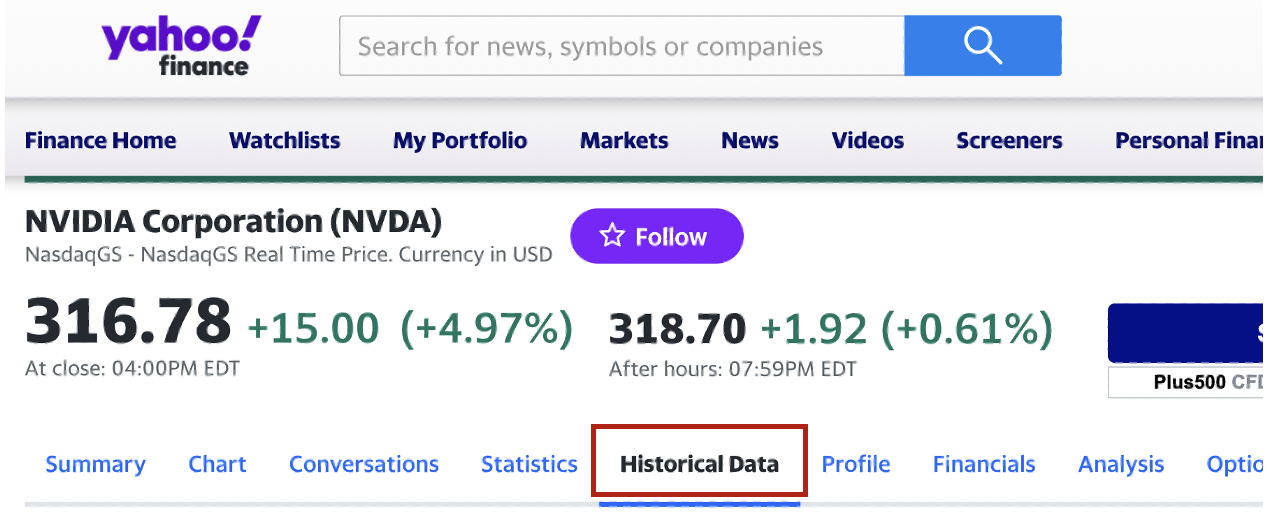
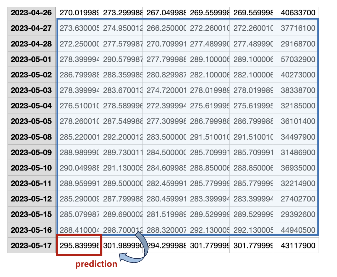
예를 들어 특정 기간의 엔비디아 주식 데이터를 다운로드 받으면 다음과 같이 Date, Open, High, Low, Close, Adj Close, Volume 등의 데이터가 CSV 포맷으로 나온다.

이 중 수정 종가(adjusted close)는 사용하지 않을 것이므로 제거한다.
# read the csv file
stock_data = pd.read_csv('data/NVDA.csv')
stock_data.drop(['Adj Close'], axis=1, inplace=True) # delete adjusted close
여기서는 LSTM을 이용해서 시가(open)를 예측하는 것을 목표로 할 것이므로 나중에 예측값과 실제값을 비교하기 위해서 따로 떼어내서 저장한다. 그래프를 그리기 위해서 날짜(date)도 따로 저장한다.
# save original 'Open' prices for later
original_open = stock_data['Open'].values

# separate dates for future plotting
dates = pd.to_datetime(stock_data['Date'])
학습용 데이터는 Open, High, Low, Close, Volume 등 5가지다.
# variables for training
cols = list(stock_data)[1:6]

# new dataframe with only training data - 5 columns
stock_data = stock_data[cols].astype(float)
거래량(volume) 데이터와 주식 가격 데이터의 크기 차이가 상당하고, 또한 LSTM의 활성함수가 tanh와 sigmoid이므로 다음과 같이 학습용 데이터를 정규화한다.
# normalize the dataset
scaler = StandardScaler()
scaler = scaler.fit(stock_data)
stock_data_scaled = scaler.transform(stock_data)
학습용 데이터와 예측의 정확도를 검증하기 위한 테스트 데이터를 9:1 비율로 나눈다.
# split to train data and test data
n_train = int(0.9*stock_data_scaled.shape[0])
train_data_scaled = stock_data_scaled[0: n_train]
train_dates = dates[0: n_train]

test_data_scaled = stock_data_scaled[n_train:]
test_dates = dates[n_train:]
주가 예측은 예측일 적전 14일간의 Open, High, Low, Close, Volume를 기반으로 당일의 시가(Open)를 예측하는 것을 목표로 한다.
따라서 데이터 구조를 LSTM의 입력과 출력에 맞게 바꿔줘야 한다.
# data reformatting for LSTM
pred_days = 1  # prediction period
seq_len = 14   # sequence length = past days for future prediction.
input_dim = 5  # input_dimension = ['Open', 'High', 'Low', 'Close', 'Volume']

trainX = []
trainY = []
testX = []
testY = []

for i in range(seq_len, n_train-pred_days +1):
    trainX.append(train_data_scaled[i - seq_len:i, 0:train_data_scaled.shape[1]])
    trainY.append(train_data_scaled[i + pred_days - 1:i + pred_days, 0])

for i in range(seq_len, len(test_data_scaled)-pred_days +1):
    testX.append(test_data_scaled[i - seq_len:i, 0:test_data_scaled.shape[1]])
    testY.append(test_data_scaled[i + pred_days - 1:i + pred_days, 0])

trainX, trainY = np.array(trainX), np.array(trainY)
testX, testY = np.array(testX), np.array(testY)
LSTM 모델은 다음과 같이 2층으로 된 stacked LSTM으로 한다. 시퀀스 길이는 14이고 1층의 은닉 상태변수의 차원은 \(\mathbf{h}_t^{(1)} \in \mathbb{R}^{64}\), 2층의 은닉 상태변수 차원은 \(\mathbf{h}_t^{(2)} \in \mathbb{R}^{32}\), 입력 변수의 차원은 \(\mathbf{x}_t \in \mathbb{R}^5\) 이다. 1층은 모든 시퀀스에서 은닉 상태를 출력해야 하기 때문에 return_sequences=True 를 사용하고, 2층은 마지막 시퀀스에서만 출력이 필요하기 때문에 이 속성을 사용하지 않는다. LSTM의 출력에 사이즈가 1인 완전연결(FC) 레이어가 연결되어 있다.
# LSTM model
model = Sequential()
model.add(LSTM(64, input_shape=(trainX.shape[1], trainX.shape[2]),
               return_sequences=True))
model.add(LSTM(32, return_sequences=False))
model.add(Dense(trainY.shape[1]))

학습 결과는 다음과 같다.

녹색은 LSTM의 학습에 사용된 시가(open) 데이터이고 빨강색은 예측값, 파랑색은 참값이다. 그나저나 엔비디아 주가가 저점 대비 많이 회복됐다(살걸...). 다음 그림은 예측 구간을 자세히 들여다 본 것이다.

꽤 정확하게 시가를 예측한 것을 볼 수 있다.
이번에는 학습된 파라미터를 저장해 두고 LSTM의 시퀀스 길이를 2로 바꾸고 실행해봤다. 2일간의 데이터만 가지고 예측하겠다는 의미다. LSTM은 시퀀스 길이에 상관없이 파라미터를 공유하기 때문에 가능한 일이다.

그러면 예측 오차가 상당히 커진다는 것을 알 수 있다.


다음은 Tensorflow 2로 작성한 LSTM 주가예측 전체 코드다.
""" LSTM stock price prediction: stacked LSTM """

# import libraries
import numpy as np
import pandas as pd
from tensorflow.keras.models import Sequential
from tensorflow.keras.layers import LSTM, Dense
from tensorflow.keras.optimizers import Adam
from sklearn.preprocessing import StandardScaler
import matplotlib.pyplot as plt

# read the csv file
stock_data = pd.read_csv('data/NVDA.csv')
stock_data.drop(['Adj Close'], axis=1, inplace=True) # delete adjusted close

# save original 'Open' prices for later
original_open = stock_data['Open'].values

# separate dates for future plotting
dates = pd.to_datetime(stock_data['Date'])

# variables for training
cols = list(stock_data)[1:6]

# new dataframe with only training data - 5 columns
stock_data = stock_data[cols].astype(float)

# normalize the dataset
scaler = StandardScaler()
scaler = scaler.fit(stock_data)
stock_data_scaled = scaler.transform(stock_data)

# split to train data and test data
n_train = int(0.9*stock_data_scaled.shape[0])
train_data_scaled = stock_data_scaled[0: n_train]
train_dates = dates[0: n_train]

test_data_scaled = stock_data_scaled[n_train:]
test_dates = dates[n_train:]
# print(test_dates.head(5))

# data reformatting for LSTM
pred_days = 1  # prediction period
seq_len = 14   # sequence length = past days for future prediction.
input_dim = 5  # input_dimension = ['Open', 'High', 'Low', 'Close', 'Volume']

trainX = []
trainY = []
testX = []
testY = []

for i in range(seq_len, n_train-pred_days +1):
    trainX.append(train_data_scaled[i - seq_len:i, 0:train_data_scaled.shape[1]])
    trainY.append(train_data_scaled[i + pred_days - 1:i + pred_days, 0])

for i in range(seq_len, len(test_data_scaled)-pred_days +1):
    testX.append(test_data_scaled[i - seq_len:i, 0:test_data_scaled.shape[1]])
    testY.append(test_data_scaled[i + pred_days - 1:i + pred_days, 0])

trainX, trainY = np.array(trainX), np.array(trainY)
testX, testY = np.array(testX), np.array(testY)

# print(trainX.shape, trainY.shape)
# print(testX.shape, testY.shape)

# LSTM model
model = Sequential()
model.add(LSTM(64, input_shape=(trainX.shape[1], trainX.shape[2]), # (seq length, input dimension)
               return_sequences=True))
model.add(LSTM(32, return_sequences=False))
model.add(Dense(trainY.shape[1]))

model.summary()

# specify your learning rate
learning_rate = 0.01
# create an Adam optimizer with the specified learning rate
optimizer = Adam(learning_rate=learning_rate)
# compile your model using the custom optimizer
model.compile(optimizer=optimizer, loss='mse')

# Try to load weights
try:
    model.load_weights('./save_weights/lstm_weights.h5')
    print("Loaded model weights from disk")
except:
    print("No weights found, training model from scratch")
    # Fit the model
    history = model.fit(trainX, trainY, epochs=30, batch_size=32,
                    validation_split=0.1, verbose=1)
    # Save model weights after training
    model.save_weights('./save_weights/lstm_weights.h5')

    plt.plot(history.history['loss'], label='Training loss')
    plt.plot(history.history['val_loss'], label='Validation loss')
    plt.legend()
    plt.show()


# prediction
prediction = model.predict(testX)
print(prediction.shape, testY.shape)

# generate array filled with means for prediction
mean_values_pred = np.repeat(scaler.mean_[np.newaxis, :], prediction.shape[0], axis=0)

# substitute predictions into the first column
mean_values_pred[:, 0] = np.squeeze(prediction)

# inverse transform
y_pred = scaler.inverse_transform(mean_values_pred)[:,0]
print(y_pred.shape)

# generate array filled with means for testY
mean_values_testY = np.repeat(scaler.mean_[np.newaxis, :], testY.shape[0], axis=0)

# substitute testY into the first column
mean_values_testY[:, 0] = np.squeeze(testY)

# inverse transform
testY_original = scaler.inverse_transform(mean_values_testY)[:,0]
print(testY_original.shape)

# plotting
plt.figure(figsize=(14, 5))

# plot original 'Open' prices
plt.plot(dates, original_open, color='green', label='Original Open Price')

# plot actual vs predicted
plt.plot(test_dates[seq_len:], testY_original, color='blue', label='Actual Open Price')
plt.plot(test_dates[seq_len:], y_pred, color='red', linestyle='--', label='Predicted Open Price')
plt.xlabel('Date')
plt.ylabel('Open Price')
plt.title('Original, Actual and Predicted Open Price')
plt.legend()
plt.show()

# Calculate the start and end indices for the zoomed plot
zoom_start = len(test_dates) - 50
zoom_end = len(test_dates)

# Create the zoomed plot
plt.figure(figsize=(14, 5))

# Adjust the start index for the testY_original and y_pred arrays
adjusted_start = zoom_start - seq_len

plt.plot(test_dates[zoom_start:zoom_end],
         testY_original[adjusted_start:zoom_end - zoom_start + adjusted_start],
         color='blue',
         label='Actual Open Price')

plt.plot(test_dates[zoom_start:zoom_end],
         y_pred[adjusted_start:zoom_end - zoom_start + adjusted_start ],
         color='red',
         linestyle='--',
         label='Predicted Open Price')

plt.xlabel('Date')
plt.ylabel('Open Price')
plt.title('Zoomed In Actual vs Predicted Open Price')
plt.legend()
plt.show()
'AI 딥러닝 > Sequence' 카테고리의 다른 글
| [seq2seq] 어텐션이 포함된 seq2seq 모델 (0) | 2023.08.23 |
|---|---|
| [seq2seq] 간단한 seq2seq 모델 구현 (0) | 2023.08.17 |
| [LSTM] LSTM-AE를 이용한 시퀀스 데이터 이상 탐지 (0) | 2023.05.31 |
| [LSTM] TF2에서 단방향 LSTM 모델 구현 - 2 (0) | 2022.07.23 |
| [LSTM] TF2에서 단방향 LSTM 모델 구현 - 1 (0) | 2022.07.21 |


댓글