최적유도법칙과 비례항법유도 (PNG)

최종 속도가 설정된 최적유도법칙(https://pasus.tistory.com/293)과 최종 속도가 설정되지 않은 최적유도법칙(https://pasus.tistory.com/294)을 '유도'해 보았다. 편의상 표적이 고정된 경우와 표적이 등속 운동을 하는 경우를 분리하여 각각의 최적유도법칙을 다시 써 보겠다.

먼저 표적이 정지 고정된 경우의 비행체의 운동방정식과 최적 유도법칙은 다음과 같다.

 

$$\begin{array}{r}\text{(1)}& & {\dot{\mathbf{r}}}_m={\mathbf{v}}_m\\ & {\dot{\mathbf{v}}}_m={\mathbf{g}}_m+{\mathbf{a}}_m\\ \\ \\ \text{(2)}& & {\mathbf{a}}_{mV}(t)=\frac{6}{t_{go}^2}({\mathbf{r}}_f-({\mathbf{r}}_m(t)+t_{go}{\mathbf{v}}_m(t)))-\frac{2}{t_{go}}({\mathbf{v}}_f-{\mathbf{v}}_m(t))-{\mathbf{g}}_m\\ \text{(3)}& & {\mathbf{a}}_{mF}(t)=\frac{3}{t_{go}^2}({\mathbf{r}}_f-({\mathbf{r}}_m(t)+t_{go}{\mathbf{v}}_m(t)+\frac{t_{go}^2}{2}{\mathbf{g}}_m))\end{array}$$

 

여기서 ${\mathbf{r}}_m,{\mathbf{v}}_m$ 은 관성 좌표계에 대한 비행체의 위치벡터와 속도벡터다. ${\mathbf{r}}_f$ 는 관성 좌표계에 대한 표적의 위치벡터, ${\mathbf{v}}_f$ 는 비행체의 최종 속도벡터 설정값이다. 윈하는 최종 타격각도(impact angle)에 따라 이 값의 크기와 방향을 설정할 수 있다. ${\mathbf{a}}_{mV}$ 는 최종 속도가 설정된 최적 가속도 명령값이고 ${\mathbf{a}}_{mF}(t)$ 는 최종 속도가 자유(free)인 최적 가속도 명령값이다.

 

 

표적이 등속 운동하는 경우의 비행체와 표적 간의 상대 운동방정식과 최적 유도법칙은 다음과 같다.

 

$$\begin{array}{r}\text{(4)}& & {\dot{\mathbf{r}}}_m={\mathbf{v}}_m\\ & {\dot{\mathbf{v}}}_m=-{\mathbf{g}}_m-{\mathbf{a}}_m\\ \\ \\ \text{(5)}& & {\mathbf{a}}_{mV}(t)=\frac{6}{t_{go}^2}(\mathbf{r}(t)+t_{go}\mathbf{v}(t))+\frac{2}{t_{go}}({\mathbf{v}}_{rf}-\mathbf{v}(t))-{\mathbf{g}}_m\\ \text{(6)}& & {\mathbf{a}}_{mF}(t)=\frac{3}{t_{go}^2}(\mathbf{r}(t)+t_{go}\mathbf{v}(t)-\frac{t_{go}^2}{2}{\mathbf{g}}_m)\end{array}$$

 

여기서 $\mathbf{r}={\mathbf{r}}_T-{\mathbf{r}}_m,\mathbf{v}={\mathbf{v}}_T-{\mathbf{v}}_m$ 은 각각 표적과 비행체의 상대 위치벡터, 상대 속도벡터다. ${\mathbf{v}}_{rf}$ 는 표적과 비행체의 최종 상대 속도벡터 설정값이다. ${\mathbf{a}}_{mV}$ 는 최종 속도가 설정된 최적 가속도 명령값이고 ${\mathbf{a}}_{mF}(t)$ 는 최종 속도가 자유(free)인 최적 가속도 명령값이다.

 

 

만약 ${\mathbf{v}}_{rf}={\mathbf{v}}_T-{\mathbf{v}}_f$ 로 놓는다면,

 

$$\begin{array}{r}\text{(7)}& {\mathbf{v}}_{rf}-\mathbf{v}(t)& ={\mathbf{v}}_T-{\mathbf{v}}_f-({\mathbf{v}}_T-{\mathbf{v}}_m)\\ & ={\mathbf{v}}_m-{\mathbf{v}}_f\end{array}$$

 

가 된다. 여기서 ${\mathbf{v}}_f$ 는 비행체의 최종 속도벡터 설정값이다. 그러면 식 (5)를 다음과 같이 수정할 수 있다.

 

$$\begin{array}{}\text{(8)}& {\mathbf{a}}_{mV}(t)=\frac{6}{t_{go}^2}(\mathbf{r}(t)+t_{go}\mathbf{v}(t))-\frac{2}{t_{go}}({\mathbf{v}}_f-{\mathbf{v}}_m(t))-{\mathbf{g}}_m\end{array}$$

 

상대 운동방정식 (4)와 최적 유도법칙 (6), (8)에서 표적 위치벡터와 속도벡터를 ${\mathbf{r}}_T(t)={\mathbf{r}}_f,{\mathbf{v}}_T(t)=0$ 으로 놓으면 표적이 고정된 운동방정식 (1)과 최적 유도법칙 (2), (3)이 된다.

 

 

이제 최적 유도법칙과 전통적인 비례항법유도(PNG, proportional navigation guidance) 법칙을 비교해 보고자 한다.

중력 가속도가 $0$ 인 가정하에서 TPNG(True PNG)는 다음과 같이 주어진다.

 

$$\begin{array}{}\text{(9)}& {\mathbf{a}}_{TPNG}=N\mathbf{\Omega }\times V_c{\mathbf{s}}_1\end{array}$$

 

여기서 $N$ 은 항법유도상수, ${\mathbf{s}}_1$ 은 비행체와 표적을 잇는 가시선(LOS, line-of-sight)의 단위벡터, $\mathbf{\Omega }$ 는 LOS 각속도(angular velocity) 벡터, $V_c$ 는 접근속력(closing speed)으로서 $V_c=-\dot{r}$ 이다. $r$ 은 비행체에서 표적까지의 거리로서 상대 위치벡터는 $\mathbf{r}=r{\mathbf{s}}_1$ 로 주어진다.

LOS 각속도 벡터는 다음과 같이 계산된다.

 

$$\begin{array}{}\text{(10)}& \mathbf{\Omega }=\frac{\mathbf{r}\times \mathbf{v}}{r^2}\end{array}$$

 

$\mathbf{b}\times (\mathbf{c}\times \mathbf{d})=(\mathbf{b}\cdot \mathbf{d})\mathbf{c}-(\mathbf{b}\cdot \mathbf{c})\mathbf{d}$ 의 관계식을 이용하면, 식 (9)는

 

$$\begin{array}{r}\text{(11)}& {\mathbf{a}}_{TPNG}& =N\frac{(\mathbf{r}\times \mathbf{v})}{r^2}\times V_c{\mathbf{s}}_1\\ & =\frac{N}{r^2}[V_c({\mathbf{s}}_1^T\mathbf{r})\mathbf{v}-V_c({\mathbf{s}}_1^T\mathbf{v})\mathbf{r}]\end{array}$$

 

이 된다. 여기서 ${\mathbf{s}}_1^T\mathbf{r}=r,{\mathbf{s}}_1^T\mathbf{v}=\dot{r}=-V_c$ 이므로 위 식에 대입하면,

 

$$\begin{array}{r}\text{(12)}& {\mathbf{a}}_{TPNG}& =\frac{N}{r^2}[r{V}_c\mathbf{v}+V_c^2\mathbf{r}]\\ & =N[\frac{V_c^2}{r^2}\mathbf{r}+\frac{V_c}{r}\mathbf{v}]\end{array}$$

 

이 된다. 그런데 만약 다음 관계식이 성립한다면,

 

$$\begin{array}{}\text{(13)}& \frac{r}{V_c}\approx t_{go}\end{array}$$

 

식 (12)는 다음과 같이 된다.

 

$$\begin{array}{r}\text{(14)}& {\mathbf{a}}_{TPNG}& =N[\frac{1}{t_{go}^2}\mathbf{r}+\frac{1}{t_{go}}\mathbf{v}]\\ & =\frac{N}{t_{go}^2}(\mathbf{r}(t)+t_{go}\mathbf{v}(t))\end{array}$$

 

식 (14)에 의하면 중력 가속도가 $0$ 인 가정하에서 식 (6)의 최적유도법칙은 $N=3$ 인 TPNG 식 (9)로 표현할 수 있음을 알 수 있다. TPNG에서 중력 가속도를 보상한다면(https://pasus.tistory.com/250) 다음과 같이 최적유도법칙을 TPNG로 근사할 수 있다.

 

$$\begin{array}{}\text{(15)}& {\mathbf{a}}_{mF}\approx {\mathbf{a}}_{TPNG}=3\mathbf{\Omega }\times V_c{\mathbf{s}}_1-{\mathbf{g}}_m\end{array}$$

 

 

 

이제 몇가지 시나리오에 대해서 시뮬레이션을 통하여 유도법칙 (2), (3), (6), (8), (15)를 검증해보자. 사용한 TPNG 코드는 다음과 같다.

 

def tpng(N, OmL, Vc, LOS_hat):
    a_cmd = N * Vc * np.cross(OmL, LOS_hat) - np.array([0,0,-g])
    a_cmd_mag = np.sqrt(a_cmd.dot(a_cmd))
    if a_cmd_mag > (g * ng_limit):
        a_cmd = (g * ng_limit) * a_cmd / a_cmd_mag

    return a_cmd

 

비교를 위해서 PPNG (pure PNG)도 적용했는데 PPNG 법칙은 다음과 같다.

 

$$\begin{array}{}\text{(16)}& {\mathbf{a}}_{PPNG}=3\mathbf{\Omega }\times {\mathbf{v}}_m-{\mathbf{g}}_p\end{array}$$

 

해당코드는 다음과 같다.

 

def ppng(N, OmL, vM):
    vM_hat = vM / np.sqrt(vM.dot(vM))
    gp = np.array([0,0,-g]) - (np.array([0,0,-g]).dot(vM_hat))*vM_hat
    a_cmd = N * np.cross(OmL, vM) - gp
    a_cmd_mag = np.sqrt(a_cmd.dot(a_cmd))
    if a_cmd_mag > (g * ng_limit):
        a_cmd = (g * ng_limit) * a_cmd / a_cmd_mag

    return a_cmd

 

최종 속도가 미설정된 최적유도법칙인 식 (6)을 구현한 코드는 다음과 같다.

 

def optg(N, r, v, Vc, R, t):
    #t_go = R/Vc
    t_go = tf-t
    a_cmd = N/(t_go*t_go) * (r + t_go*v) - np.array([0,0,-g])
    a_cmd_mag = np.sqrt(a_cmd.dot(a_cmd))
    if a_cmd_mag > (g * ng_limit):
        a_cmd = (g * ng_limit) * a_cmd / a_cmd_mag

    return a_cmd

 

최종 속도가 설정된 최적유도법칙인 식 (8)을 구현한 코드는 다음과 같다.

 

def optg_ivc(N, r, v, Vc, R, vF, vM, t):
    #t_go = R/Vc
    t_go = tf-t
    a_cmd = N/(t_go*t_go) * (r + t_go*v) - (2/t_go) * (vF-vM) - np.array([0,0,-g])

    a_cmd_mag = np.sqrt(a_cmd.dot(a_cmd))
    if a_cmd_mag > (g * ng_limit):
        a_cmd = (g * ng_limit) * a_cmd / a_cmd_mag

    return a_cmd

 

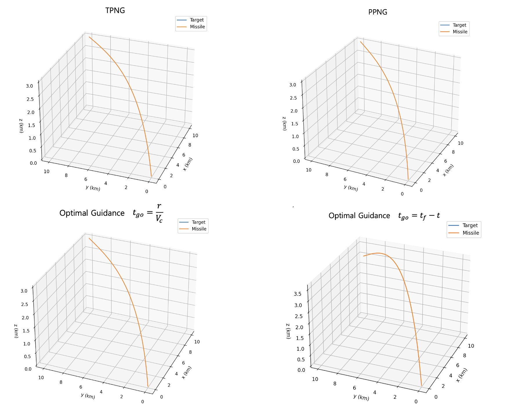
첫번째 시나리오는 표적이 위치 $x_T=10km$, $y_T=10km$, $z_T=3km$ 에 정지해 있고, 비행체는 위치 $x_M=0km$, $y_M=0km$, $z_M=0km$ 에서 속력 $V_M=400m/s$ 으로 방위각 $30$도, 고도각 $30$도로 출발하여 표적을 타격하는 것이다.

아래 그림의 첫번째 줄은 TPNG, PPNG를 적용한 결과다. 비행시간은 대략 TPNG 42초, PPNG 38초가 나왔다. 그림의 두번째 줄은 최적유도법칙 (6)을 적용한 결과다. 잔여시간(time-to-go)을 식 (13)으로 계산하면 비행시간이 대략 최적유도 40초 정도가 나오는데 왼쪽 그림이다. 최종 임무시간을 임의로 70초로 설정하여 계산한 결과는 오른쪽에 있다.

 

 

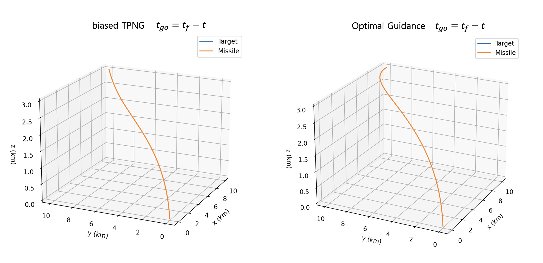
두번째 시나리오는 첫번째 시나리오와 동일하지만 표적을 최종 속도 ${\mathbf{v}}_f=[40000{]}^{T}m/s$ 로 타격하는 것이다. 아래 그림에서 왼쪽은 식 (14)와 (8)을 조합하여 만든 biased TPNG를 적용한 결과다.

 

$${\mathbf{a}}_{mV}(t)=6\mathbf{\Omega }\times V_c{\mathbf{s}}_1-\frac{2}{t_{go}}({\mathbf{v}}_f-{\mathbf{v}}_m(t))-{\mathbf{g}}_m$$

 

잔여시간을 식 (13)으로 계산하면 발산하였다. 위 식의 두번째 항의 영향으로 식 (13)의 근사식이 성립하지 않기 때문이다. 그림은 비행시간을 40초로 설정하고 잔여시간을 계산했을 때의 결과다. 표적을 타격했으나 타격각은 만족하지 못했다. 반면, 최적유도법칙을 적용했을 때는 오른쪽 그림과 같이 설정한 대로 정확히 x축 방향으로 타격했다.

 

 

세번째 시나리오는 표적이 시나리오 1과 동일한 위치에서 등속력 $V_T=300m/s$ 으로 방위각 $0$도, 고도각 $0$도로 날아가고, 비행체도 위치 $x_M=0km$, $y_M=0km$, $z_M=0km$ 에서 속력 $V_M=400m/s$ 으로 방위각 $30$도, 고도각 $30$도로 출발하여 표적을 요격하는 것이다. 아래 그림의 첫번째 줄은 TPNG, PPNG를 적용한 결과다. 비행시간은 대략 TPNG 180초, PPNG 115초가 나왔다. 그림의 두번째 줄은 최적유도법칙 (6)을 적용한 결과다. 잔여시간(time-to-go)을 식 (13)으로 계산하면 비행시간이 대략 180초 정도가 나오는데 왼쪽 그림이다. 최종 임무시간을 임의로 110초로 설정하여 계산한 결과는 오른쪽에 있다.

 

 

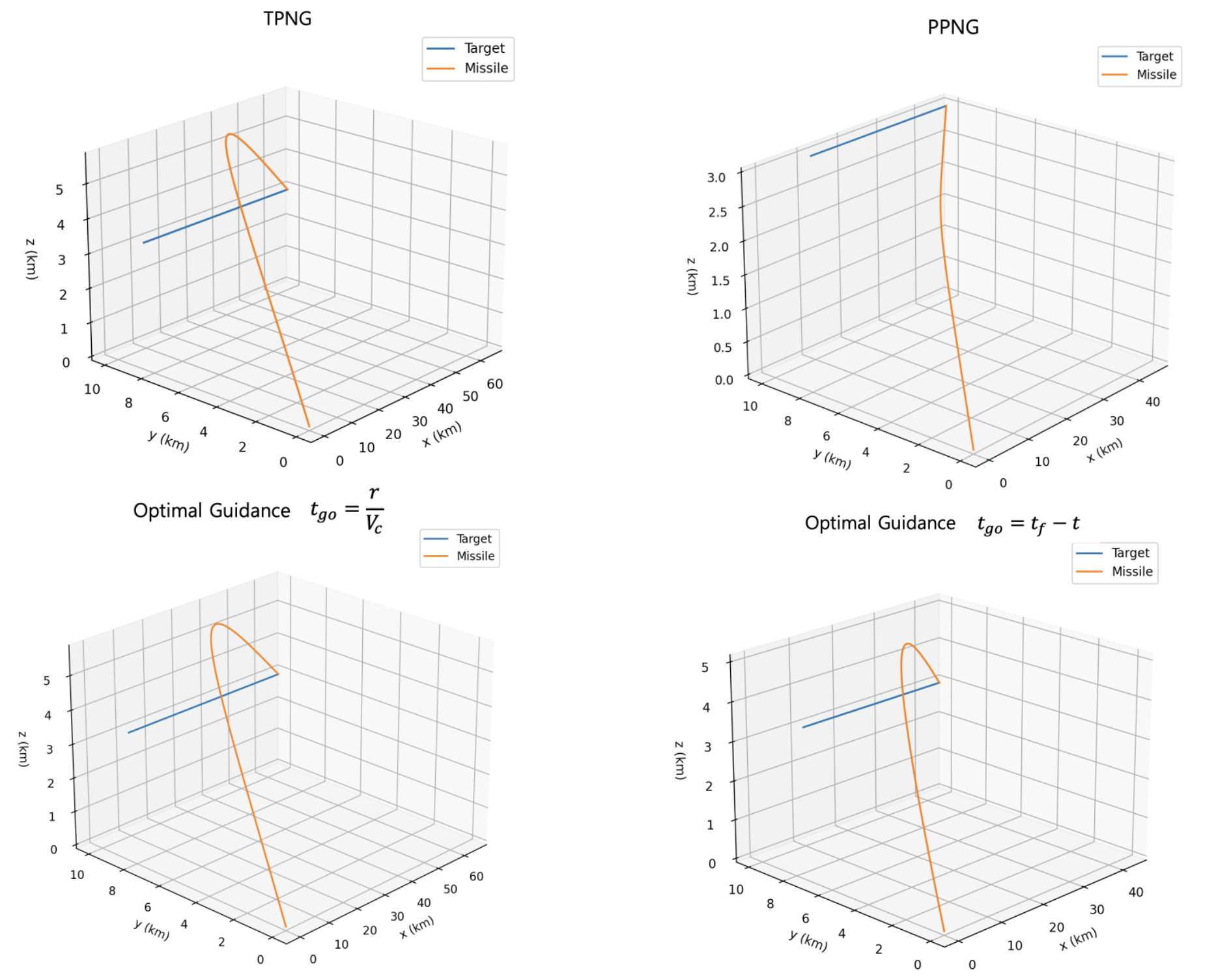
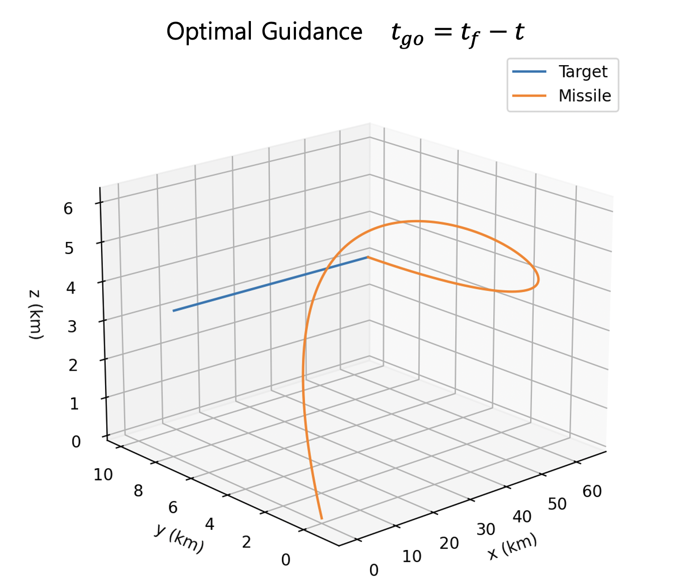
네번째 시나리오는 세번째 시나리오와 동일하지만 표적을 최종 속도 ${\mathbf{v}}_f=[04000{]}^{T}m/s$ 로 요격하는 것이다. 최적유도법칙만이 성공했으며 이 경우도 잔여시간을 최종 임무시간을 설정하고 계산한 경우에만 성공했다. 결과는 임무시간을 180초로 설정한 경우다. 설정한 대로 정확히 y축 방향으로 요격했다.

 

 

 

 

다음은 시커(seeker)의 기능을 코드로 구현한 것이다. 시커 모델에서는 LOS 각속도, LOS 방향벡터, 표적까지의 거리, 접근속도 등을 계산한다.

 

# seeker measurements or estimations
# coded by st.watermelon

from config import *
import numpy as np

def seeker_meas(rT, vT, rM, vM):
    """ relative position and velocity vector """
    rTM = rT - rM
    vTM = vT - vM

    R2 = rTM.dot(rTM)
    R = np.sqrt(R2)

    """ LOS rate """
    OmL = np.cross(rTM, vTM)/R2

    """ approaching speed """
    Vc = -rTM.dot(vTM) / R

    LOS_hat = rTM / R  # LOS direction vector

    return OmL, LOS_hat, R, Vc

 

다음은 표적과 비행체의 질점 운동모델을 코드로 구현한 것이다.

 

# 3DOF Dynamics
# coded by st.watermelon

from config import *
import numpy as np

class Dof3Dynamics:

    def __init__(self):
        pass

    """ initialization """
    def reset(self, pos, v_mag, azimuth, elevation):

        self.p_vec = np.array(pos).reshape(3, )

        vx0 = v_mag * np.cos(elevation) * np.cos(azimuth)
        vy0 = v_mag * np.cos(elevation) * np.sin(azimuth)
        vz0 = v_mag * np.sin(elevation)
        self.v_vec = np.array([vx0, vy0, vz0]).reshape(3, )

        return np.copy(self.p_vec), np.copy(self.v_vec)  # shape (3,)


    def step(self, a_cmd, option):

        """ compute numerical integration(RK4) """
        xx = np.append(self.p_vec, self.v_vec)

        k1 = dt * self.fn(xx, a_cmd, option)
        k2 = dt * self.fn(xx + dt / 2 * k1, a_cmd, option)
        k3 = dt * self.fn(xx + dt / 2 * k2, a_cmd, option)
        k4 = dt * self.fn(xx + dt * k3, a_cmd, option)
        k = (k1 + 2 * k2 + 2 * k3 + k4) / 6

        xx = xx + k

        self.p_vec = xx[0:3]
        self.v_vec = xx[3:6]

        return np.copy(self.p_vec), np.copy(self.v_vec)

    """ 3DOF dynamics """
    def fn(self, xx, ctrl, option):
        if option == 'target':
            with_g = 0
        else:
            with_g = 1

        v = xx[3:6]

        p_dot = v
        v_dot = ctrl + with_g*np.array(([0, 0, -g]))
        xx_dot = np.append(p_dot, v_dot)
        return xx_dot

 

다음은 시나리오 실행 코드이다.

 

# test guidance laws
# coded by st.watermelon

from config import *
from guidance import *
from dof3_dynamics import *
from seeker_meas import *

import numpy as np
import matplotlib.pyplot as plt

""" create target objects """
target = Dof3Dynamics()
# set initial position and velocity of target
posT = [10000, 10000, 3000]
v_magT = 300
azimuthT = 0*np.pi/180
elevationT = 0*np.pi/180

rT0, vT0 = target.reset(posT, v_magT, azimuthT, elevationT)

""" create missile objects """
missile = Dof3Dynamics()
# set position and velocity of missile
posM = [0, 0, 0]
v_magM = 400
azimuthM = 30*np.pi/180
elevationM = 30*np.pi/180
impact_dir = np.array([0, 1, 0])
impact_dir = impact_dir / np.sqrt(impact_dir.dot(impact_dir))
vF = v_magM*impact_dir

rM0, vM0 = missile.reset(posM, v_magM, azimuthM, elevationM)


""" processing """
# save the results
pos_target = []
pos_missile = []
vel_missile = []
sp_missile = []
rel_distance = []
command = []
look_angle = []
run_time = []


for k in range(100000):
    t = k*dt
    print(f't= {t:.3f}')

    """ seeker measurement """
    OmL, LOS_hat, R, Vc = seeker_meas(rT0, vT0, rM0, vM0)

    """ guidance law """
    a_cmd = optg(3, rT0-rM0, vT0-vM0, Vc, R, t)
    #a_cmd = optg_ivc(6, rT0 - rM0, vT0 - vM0, Vc, R, vF, vM0, t)

    #a_cmd = tpng(3, OmL, Vc, LOS_hat)
    #a_cmd = ppng(3, OmL, vM0)

    """ missile dynamics """
    rM, vM = missile.step(a_cmd, 'missile')

    """ target dynamics """
    a_cmd_target = np.array([0, 0, 0])
    rT, vT = target.step(a_cmd_target, 'target')


    """ collections """
    pos_target.append(rT0)
    pos_missile.append(rM0)
    vel_missile.append(vM0)
    sp_missile.append(np.sqrt(vM.dot(vM)))
    rel_distance.append(R)
    command.append(a_cmd)
    run_time.append(t)


    """ for the next step """
    rM0 = rM
    vM0 = vM
    rT0 = rT
    vT0 = vT

    """ stop condition """
    if R < 5:
        break

print(f'simulation done at time: {t:.3f} sec, and R: {R:.3f} m')

# convert lists to numpy arrays
pos_target = np.array(pos_target)
pos_missile = np.array(pos_missile)
vel_missile = np.array(vel_missile)
rel_distance = np.array(rel_distance)
command = np.array(command)
run_time = np.array(run_time)


# plot target and missile positions
fig1, ax1 = plt.subplots(subplot_kw={'projection': '3d'})
ax1.plot(pos_target[:, 0]/1000, pos_target[:, 1]/1000, pos_target[:, 2]/1000, label='Target')
ax1.plot(pos_missile[:, 0]/1000, pos_missile[:, 1]/1000, pos_missile[:, 2]/1000, label='Missile')
ax1.set_xlabel('x (km)')
ax1.set_ylabel('y (km)')
ax1.set_zlabel('z (km)')
ax1.legend()
ax1.set_title('Target and Missile Positions')

# plot relative distance
fig2, ax2 = plt.subplots()
ax2.plot(run_time, rel_distance)
ax2.set_xlabel('Time [s]')
ax2.set_ylabel('Relative Distance [m]')
ax2.set_title('Relative Distance vs Time')

# plot control commands
fig3, ax3 = plt.subplots()
ax3.plot(run_time, command[:, 0], label='a_x')
ax3.plot(run_time, command[:, 1], label='a_y')
ax3.plot(run_time, command[:, 2], label='a_z')
ax3.set_xlabel('Time [s]')
ax3.set_ylabel('Control Commands (a_cmd)')
ax3.legend()
ax3.set_title('Control Commands a_cmd vs Time')

# plot missile velocity
fig4, ax4 = plt.subplots()
ax4.plot(run_time, vel_missile[:, 0], label='vx')
ax4.plot(run_time, vel_missile[:, 1], label='vy')
ax4.plot(run_time, vel_missile[:, 2], label='vz')
ax4.set_xlabel('Time [s]')
ax4.set_ylabel('missile velocity (m/s)')
ax4.legend()
ax4.set_title('Missile Velocity')


# plot missile speed
fig5, ax5 = plt.subplots()
ax5.plot(run_time, sp_missile)
ax5.set_xlabel('Time [s]')
ax5.set_ylabel('missile velocity (m/s)')
ax5.set_title('Missile Velocity')

# display all plots
plt.show()