표준 DMD의 한 가지 제한 사항은 시스템의 운동을 바꾸거나 측정할 수 있는 외부 입력과 출력이 포함된 모델을 생성할 수 없다는 것이다.
이제 표준 DMD 방법을 확장하여 입력과 출력이 포함된 시스템 모델을 식별해 보도록 한다. 이와 같이 입출력이 포함된 확장 DMD를 DMDio (DMD with input/output)이라고 한다. 모델 입력과 출력이 포함된 시스템의 동적 특성을 이해하는 것은 제어기 설계 및 센서 배치 문제의 기본 전제 사항이다.
식별하고자 하는 미지의 이산시간 시스템이 식 (1)과 같이 표현된다고 하자.
\[ \begin{align} & \mathbf{x}_{k+1}=A \mathbf{x}_k+B \mathbf{u}_k \tag{1} \\ \\ & \mathbf{y}_k=C \mathbf{x}_k+D \mathbf{u}_k \end{align} \]
여기서 \(\mathbf{x}_k \in \mathbb{R}^n\), \(\mathbf{u}_k \in \mathbb{R}^p\), \(\mathbf{y}_k \in \mathbb{R}^q\), \(A \in \mathbb{R}^{n \times n}\), \(B \in \mathbb{R}^{n \times p}\), \(C \in \mathbb{R}^{q \times n}\), \(D \in \mathbb{R}^{q \times p}\) 이다. 입력과 출력의 차원 \(p\) 와 \(q\) 는 일반적으로 매우 작은 값으로 \(p,q≪n\) 이다.
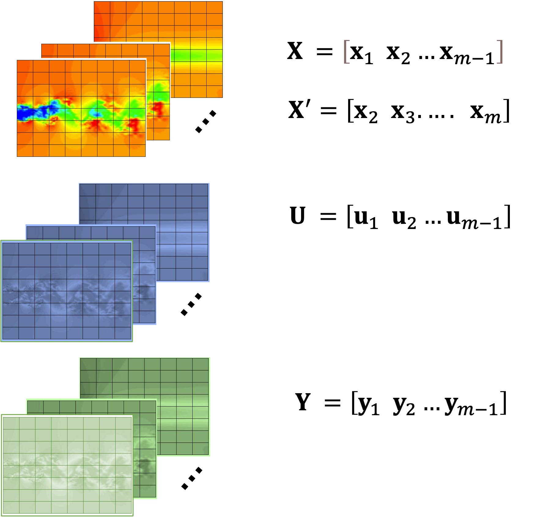
이제, 일정한 싯점에서 \(m\) 개의 상태변수 스냅샷 데이터 \(\mathbf{x}_k\) 와 \((m-1)\) 개의 입력과 출력의 스냅샷 데이터 \(\mathbf{u}_k\) 와 \(\mathbf{y}_k\) 를 수집하여 이를 다음과 같이 행렬 형태로 표현한다. 여기서 \(\mathbf{u}_k\) 는 임의의 입력이다.
\[ \begin{align} & \mathbf{X} =[\mathbf{x}_1 \ \ \ \mathbf{x}_2 \ \ \ \cdots \ \ \ \mathbf{x}_{m-1} ] \ \ \ \in \mathbb{R}^{n \times (m-1)} \tag{2} \\ \\ & \mathbf{X}' =[\mathbf{x}_2 \ \ \ \mathbf{x}_3 \ \ \ \cdots \ \ \ \mathbf{x}_m \ ] \ \ \ \ \ \in \mathbb{R}^{n \times (m-1)} \\ \\ & \mathbf{U} =[\mathbf{u}_1 \ \ \ \mathbf{u}_2 \ \ \ \cdots \ \ \ \mathbf{u}_{m-1} ] \ \ \ \in \mathbb{R}^{p \times (m-1)} \\ \\ & \mathbf{Y} =[\mathbf{y}_1 \ \ \ \mathbf{y}_2 \ \ \ \cdots \ \ \ \mathbf{y}_{m-1} ] \ \ \ \in \mathbb{R}^{q \times (m-1)} \end{align} \]
여기서 \(\mathbf{X}'\) 은 \(\mathbf{X}\) 를 한 시간스텝 만큼 시프트(shift)시킨 행렬이다.
식 (1)의 시스템 운동식을 이용하면 다음과 같은 관계식을 유도할 수 있다.
\[ \begin{align} \mathbf{X}' &= [ A\mathbf{x}_1+B\mathbf{u}_1 \ \ \ A\mathbf{x}_2+B \mathbf{u}_2 \ \ \ \cdots \ \ \ A\mathbf{x}_{m-1}+B\mathbf{u}_{m-1} \ ] \tag{3} \\ \\ &=A \mathbf{X}+B \mathbf{U} \\ \\ \mathbf{Y} &= [ C\mathbf{x}_1+D\mathbf{u}_1 \ \ \ C\mathbf{x}_2+D\mathbf{u}_2 \ \ \ \cdots \ \ \ C\mathbf{x}_{m-1}+D \mathbf{u}_{m-1} \ ] \\ \\ &= C \mathbf{X}+D \mathbf{U} \end{align} \]
식 (3)을 한 개의 행렬식으로 표현하면 다음과 같다.
\[ \begin{bmatrix} \mathbf{X}'\\ \mathbf{Y} \end{bmatrix} = \begin{bmatrix} A & B \\ C & D \end{bmatrix} \begin{bmatrix} \mathbf{X} \\ \mathbf{U} \end{bmatrix} \tag{4} \]
또는 더 간단하게
\[ \mathbf{Z}= \mathbf{G} \mathbf{\Omega} \tag{5} \]
로 표기할 수 있다. 여기서 \(\mathbf{\Omega}= \begin{bmatrix} \mathbf{X} \\ \mathbf{U} \end{bmatrix} \in \mathbb{R}^{(n+p) \times (m-1)}\) 는 상태와 입력의 스냅샷 정보가 모두 담긴 행렬이고, \(\mathbf{Z}= \begin{bmatrix} \mathbf{X}' \\ \mathbf{Y} \end{bmatrix} \in \mathbb{R}^{(n+q) \times (m-1)}\) 는 상태와 출력의 스냅샷 정보가 담긴 행렬, \(\mathbf{G}= \begin{bmatrix} A & B \\ C & D \end{bmatrix} \in \mathbb{R}^{(n+q) \times (n+p)}\) 는 시스템의 구성 행렬이 조합된 것으로서 DMDio가 식별하고자 하는 행렬이다.
표준 DMD와 마찬가지로 \(\mathbf{G}\) 는 다음과 같이 프로베니우스(Frobenius) 놈이 최소화되도록 계산할 수 있다.
\[ \mathbf{G}= \arg \min_{\mathbf{G}} \lVert \mathbf{Z}- \mathbf{G} \mathbf{\Omega} \rVert _F = \mathbf{Z} \mathbf{\Omega}^+ \tag{6} \]
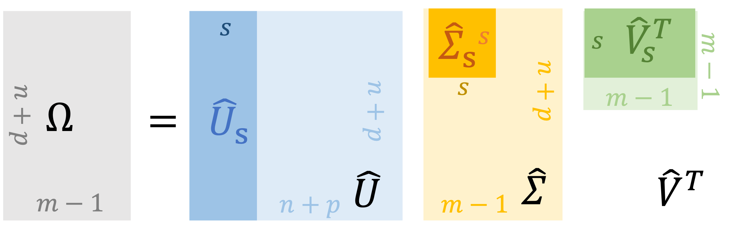
여기서 \(\mathbf{\Omega}^+\) 는 무어-펜로즈 유사 역행렬 (Moore-Penrose pseudo inverse matrix)이다. 유사 역행렬은 특이값 분해(SVD, singular value decomposition)를 이용해서 계산할 수 있다. 행렬 \(\mathbf{\Omega}\) 의 SVD는 다음과 같다.
\[ \begin{align} \mathbf{\Omega} &= \hat{U} \hat{\Sigma} \hat{V}^T = \begin{bmatrix} \hat{U}_s & \hat{U}_{rem} \end{bmatrix} \begin{bmatrix} \hat{\Sigma}_s & 0 \\ 0 & \hat{\Sigma}_{rem} \end{bmatrix} \begin{bmatrix} \hat{V}_s^T \\ \hat{V}_{rem}^T \end{bmatrix} \tag{7} \\ \\ & \approx \hat{U}_s \hat{\Sigma}_s \hat{V}_s^T \end{align} \]
여기서 \( \hat{U} \in \mathbb{R}^{(n+p) \times (n+p)}\), \(\hat{\Sigma} \in \mathbb{R}^{(n+p) \times (m-1)}\), \(\hat{V} \in \mathbb{R}^{(m-1) \times (m-1)}\), \(\hat{U}_s \in \mathbb{R}^{(n+p) \times s}\), \(\hat{\Sigma}_s \in \mathbb{R}^{s \times s}\), \(\hat{V}_s \in \mathbb{R}^{(m-1) \times s}\) 이다. \(s\) 는 절단값(truncation value)으로서 설계 변수가 된다.
그러면 유사 역행렬 \(\mathbf{\Omega}^+\) 은 다음과 같이 근사적으로 계산할 수 있다.
\[ \mathbf{\Omega}^+ \approx \hat{V}_s \hat{\Sigma}_s^{-1} \hat{U}_s^T \ \ \ \in \mathbb{R}^{(m-1) \times (n+p)} \tag{8} \]
식 (8)을 (6)에 대입하면 \(\mathbf{G}\) 는 다음과 같이 된다.
\[ \begin{align} \mathbf{G} &= \begin{bmatrix} A & B \\ C & D \end{bmatrix} \approx \mathbf{Z} \hat{V}_s \hat{\Sigma}_s^{-1} \hat{U}_s^T \tag{9} \\ \\ &= \begin{bmatrix} \mathbf{X}' \\ \mathbf{Y} \end{bmatrix} \begin{bmatrix} \hat{V}_s \hat{\Sigma}_s^{-1} \hat{U}_1^T & \hat{V}_s \hat{\Sigma}_s^{-1} \hat{U}_2^T \end{bmatrix} \\ \\ &= \begin{bmatrix} \mathbf{X}' \hat{V}_s \hat{\Sigma}_s^{-1} \hat{U}_1^T & \mathbf{X}' \hat{V}_s \hat{\Sigma}_s^{-1} \hat{U}_2^T \\ \mathbf{Y} \hat{V}_s \hat{\Sigma}_s^{-1} \hat{U}_1^T & \mathbf{Y} \hat{V}_s \hat{\Sigma}_s^{-1} \hat{U}_2^T \end{bmatrix} \end{align} \]
따라서 행렬 \(A, \ B, \ C, \ D\) 는 각각 다음과 같이 식별할 수 있다.
\[ \begin{align} & A= \mathbf{X}' \hat{V}_s \hat{\Sigma}_s^{-1} \hat{U}_1^T \tag{10} \\ \\ & B=\mathbf{X}' \hat{V}_s \hat{\Sigma}_s^{-1} \hat{U}_2^T \\ \\ & C= \mathbf{Y} \hat{V}_s \hat{\Sigma}_s^{-1} \hat{U}_1^T \\ \\ & D=\mathbf{Y} \hat{V}_s \hat{\Sigma}_s^{-1} \hat{U}_2^T \end{align} \]
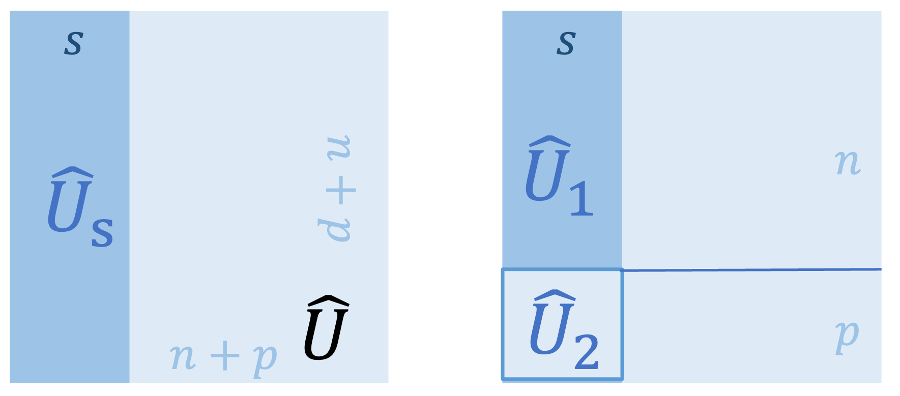
여기서 \(\hat{U}_s^T = \begin{bmatrix} \hat{U}_1^T & \hat{U}_2^T \end{bmatrix} \) 이고 \(\hat{U}_1 \in \mathbb{R}^{n \times s}\), \(\hat{U}_2 \in \mathbb{R}^{p \times s}\) 이다.
표준 DMD 에서와 마찬가지로 \(n\) 차 모델을 \(r\) 차 축소 모델 (ROM, reduced order model)로 근사화 하자. 여기서 r≪n이다. 모델 축소화에서 일반적으로 쓰이는 방법은 투사(projection) 방법이다. 선형 기저 변환(basis transformation)을 통해서 \(n\)차 벡터 \(\mathbf{x}_k\) 를 \(r\) 차 벡터 \(\tilde{\mathbf{x}}_k\) 로 축소 변환한다.
\[ \mathbf{x}_k=P \tilde{\mathbf{x}}_k \tag{11} \]
여기서 \(P \in \mathbb{R}^{n \times r}\) 는 변환 행렬로서 \(P^T P=I\) 를 만족한다.
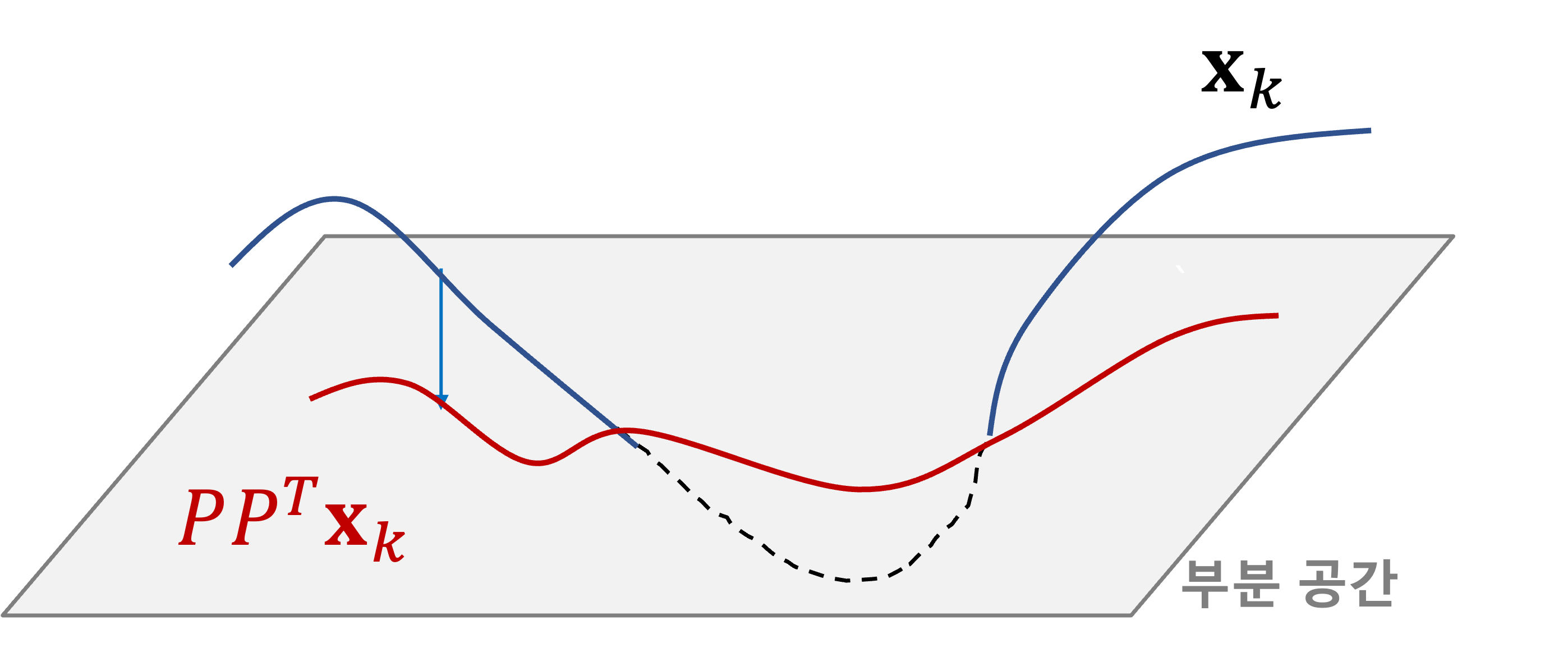
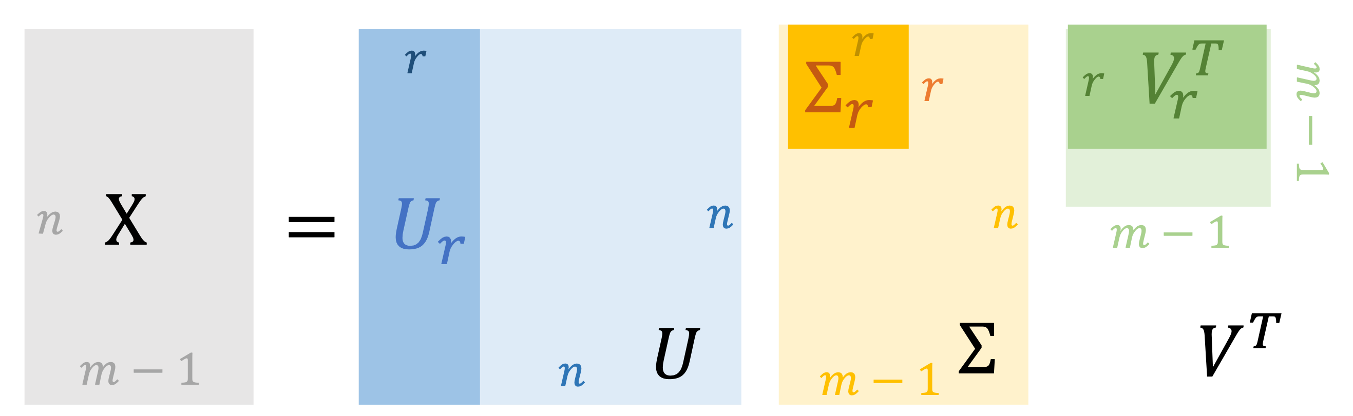
투사 오차(prediction error)를 최소화하도록 기저 좌표축을 결정하기 위해서 스냅샷 POD(proper orthogonal decomposition) 알고리즘을 이용하여 변환 행렬을 결정하도록 한다. 상태변수의 변환 행렬이므로 표준 DMD와 마찬가지로 행렬 \(\mathbf{X}\) 의 SVD의 왼쪽 특이 벡터(left singular vector)를 변환 행렬로 사용해야 한다. 따라서 \(\mathbf{\Omega}\) 에 이어서 행렬 \(\mathbf{X}\) 의 SVD가 더 필요하다.
\[ \begin{align} \mathbf{X} &= U \Sigma V^T = \begin{bmatrix} U_r & U_{rem} \end{bmatrix} \begin{bmatrix} \Sigma_r & 0 \\ 0 & \Sigma_{rem} \end{bmatrix} \begin{bmatrix} V_r^T \\ V_{rem}^T \end{bmatrix} \tag{12} \\ \\ & \approx U_r \Sigma_r V_r^T \end{align} \]
여기서 \(U \in \mathbb{R}^{n \times n}\), \(\Sigma \in \mathbb{R}^{n \times (m-1)}\), \( V \in \mathbb{R}^{(m-1) \times (m-1)}\), \(U_r \in \mathbb{R}^{n \times r}\), \(\Sigma_r \in \mathbb{R}^{r \times r}\), \(V_r \in R^{(m-1) \times r}\) 이다. \(r\) 은 시스템의 차원을 \(n\) 에서 \(r\) 로 줄이기 위한 절단값(truncation value)으로서 설계 변수가 된다.
이제 \(P=U_r\) 로 놓고 식 (12)를 식 (1)에 대입하면 다음과 같이 된다.
\[ \begin{align} & \tilde{\mathbf{x}}_{k+1}=U_r^T \mathbf{x}_{k+1}=U_r^T AU_r \tilde{\mathbf{x}}_k+U_r^T B \mathbf{u}_k \tag{13} \\ \\ & \mathbf{y}_k=CU_r \tilde{\mathbf{x}}_k+D \mathbf{u}_k \end{align} \]
여기서 식 (10)을 위 식에 대입하면 다음과 같이 된다.
\[ \begin{align} \tilde{\mathbf{x}}_{k+1} &= U_r^T \mathbf{X}' \hat{V}_s \hat{\Sigma}_s^{-1} \hat{U}_1^T U_r \tilde{\mathbf{x}}_k+U_r^T \mathbf{X}' \hat{V}_s \hat{\Sigma}_s^{-1} \hat{U}_2^T \mathbf{u}_k \tag{14}\\ \\ &= \tilde{A} \tilde{\mathbf{x}}_k+ \tilde{B} \mathbf{u}_k \\ \\ \mathbf{y}_k &= \mathbf{Y} \hat{V}_s \hat{\Sigma}_s^{-1} \hat{U}_1^T U_r \tilde{\mathbf{x}}_k+D\mathbf{u}_k \\ \\ &= \tilde{C} \tilde{\mathbf{x}}_k+D\mathbf{u}_k \end{align} \]
여기서
\[ \begin{align} & \tilde{A} = U_r^T \mathbf{X}' \hat{V}_s \hat{\Sigma}_s^{-1} \hat{U}_1^T U_r \ \ \ \in \mathbb{R}^{r \times r} \\ \\ & \tilde{B} = U_r^T \mathbf{X}' \hat{V}_s \hat{\Sigma}_s^{-1} \hat{U}_2^T \ \ \ \in \mathbb{R}^{r \times p} \\ \\ & \tilde{C} = \mathbf{Y} \hat{V}_s \hat{\Sigma}_s^{-1} \hat{U}_1^T U_r \ \ \ \in \mathbb{R}^{q \times r} \end{align} \]
시스템 행렬 \(A\) 의 동특성을 파악하기 위해서 표준 DMD과 마찬가지로 축소 시스템 행렬 \(\tilde{A}\) 의 고유값 \(\lambda_i\) 와 고유벡터 \(\mathbf{w}_i\) 를 먼저 계산한다. 축소 시스템 행렬 \(\tilde{A}\) 의 고유값과 고유벡터 식은 다음과 같다.
\[ \begin{align} \tilde{A} \mathbf{w}_i &= U_r^T \mathbf{X}' \hat{V}_s \hat{\Sigma}_s^{-1} \hat{U}_1^T U_r \mathbf{w}_i \tag{15} \\ \\ &= \lambda_i \mathbf{w}_i , \ \ \ \ \ i=1, \ ..., \ r \end{align} \]
이제 벡터 \(\phi_i\) 를 다음과 같이 정의하자.
\[ \phi_i = \mathbf{X}' \hat{V}_s \hat{\Sigma}_s^{-1} \hat{U}_1^T U_r \mathbf{w}_i \tag{16} \]
그러면 식 (16)은 다음과 같이 된다.
\[ U_r^T \phi_i= \lambda_i \mathbf{w}_i \tag{17} \]
위 식의 양변에 \( \mathbf{X}' \hat{V}_s \hat{\Sigma}_s^{-1} \hat{U}_1^T U_r \) 을 곱하면,
\[ \mathbf{X}' \hat{V}_s \hat{\Sigma}_s^{-1} \hat{U}_1^T U_r U_r^T \phi_i= \lambda_i \mathbf{X}' \hat{V}_s \hat{\Sigma}_s^{-1} \hat{U}_1^T U_r \mathbf{w}_i \tag{18} \]
이 된다. 근사적으로
\[ \mathbf{X}' \hat{V}_s \hat{\Sigma}_s^{-1} \hat{U}_1^T U_r U_r^T \approx \mathbf{X}' \hat{V}_s \hat{\Sigma}_s^{-1} \hat{U}_1^T \]
이므로 식 (10)과 (16)에 의하면 위 식은 다음과 같이 된다.
\[ A \phi_i= \lambda_i \phi_i , \ \ \ \ \ i=1, \ ..., \ r \tag{19} \]
위 식은 행렬 \(A\) 의 고유값과 고유벡터 식이다. 따라서 원래 시스템 \(A\) 와 축소 시스템 \(\tilde{A}\) 의 고유값은 근사적으로 같고 고유벡터는 식 (16)의 관계가 성립한다는 것을 알 수 있다. 원래 시스템 \(A\) 의 고유벡터 \(\phi_i\) 를 DMD 모드라고 한다.
DMDio 방법을 정리하면 다음과 같다.
1. 먼저 \(m\) 개의 스냅샷 데이터 \(\mathbf{x}_k\) 와 \((m-1)\) 개의 스냅샷 데이터 \(\mathbf{u}_k\), \(\mathbf{y}_k\) 를 수집하여 이를 다음과 같이 행렬 형태로 표현한다.
\[ \begin{align} & \mathbf{X} =[\mathbf{x}_1 \ \ \ \mathbf{x}_2 \ \ \ \cdots \ \ \ \mathbf{x}_{m-1} ] \ \ \ \in \mathbb{R}^{n \times (m-1)} \\ \\ & \mathbf{X}' =[\mathbf{x}_2 \ \ \ \mathbf{x}_3 \ \ \ \cdots \ \ \ \mathbf{x}_m \ ] \ \ \ \ \ \in \mathbb{R}^{n \times (m-1)} \\ \\ & \mathbf{U} =[\mathbf{u}_1 \ \ \ \mathbf{u}_2 \ \ \ \cdots \ \ \ \mathbf{u}_{m-1} ] \ \ \ \in \mathbb{R}^{p \times (m-1)} \\ \\ & \mathbf{Y} =[\mathbf{y}_1 \ \ \ \mathbf{y}_2 \ \ \ \cdots \ \ \ \mathbf{y}_{m-1} ] \ \ \ \in \mathbb{R}^{q \times (m-1)} \end{align} \]
2. 행렬 \(\mathbf{\Omega}= \begin{bmatrix} \mathbf{X} \\ \mathbf{U} \end{bmatrix}\) 의 SVD를 계산한다.
\[ \begin{align} \mathbf{\Omega} &= \hat{U} \hat{\Sigma} \hat{V}^T = \begin{bmatrix} \hat{U}_s & \hat{U}_{rem} \end{bmatrix} \begin{bmatrix} \hat{\Sigma}_s & 0 \\ 0 & \hat{\Sigma}_{rem} \end{bmatrix} \begin{bmatrix} \hat{V}_s^T \\ \hat{V}_{rem}^T \end{bmatrix} \\ \\ & \approx \hat{U}_s \hat{\Sigma}_s \hat{V}_s^T \\ \\ & = \begin{bmatrix} \hat{U}_1 \\ \hat{U}_2 \end{bmatrix} \hat{\Sigma}_s \hat{V}_s^T \end{align} \]
3. 행렬 \(\mathbf{X}\) 의 SVD를 계산한다.
\[ \begin{align} \mathbf{X} &= U \Sigma V^T = \begin{bmatrix} U_r & U_{rem} \end{bmatrix} \begin{bmatrix} \Sigma_r & 0 \\ 0 & \Sigma_{rem} \end{bmatrix} \begin{bmatrix} V_r^T \\ V_{rem}^T \end{bmatrix} \\ \\ & \approx U_r \Sigma_r V_r^T \end{align} \]
4. 축소 시스템을 구한다.
\[ \begin{align} & \tilde{\mathbf{x}}_{k+1} = \tilde{A} \tilde{\mathbf{x}}_k+ \tilde{B} \mathbf{u}_k \\ \\ & \mathbf{y}_k = \tilde{C} \tilde{\mathbf{x}}_k+D\mathbf{u}_k \\ \\ & \ \ \ \ \mathbf{x}_k = U_r \tilde{\mathbf{x}}_k \\ & \ \ \ \ \tilde{A} = U_r^T \mathbf{X}' \hat{V}_s \hat{\Sigma}_s^{-1} \hat{U}_1^T U_r \\ & \ \ \ \ \tilde{B} = U_r^T \mathbf{X}' \hat{V}_s \hat{\Sigma}_s^{-1} \hat{U}_2^T \\ & \ \ \ \ \tilde{C} = \mathbf{Y} \hat{V}_s \hat{\Sigma}_s^{-1} \hat{U}_1^T U_r \\ & \ \ \ \ D = \mathbf{Y} \hat{V}_s \hat{\Sigma}_s^{-1} \hat{U}_2^T \end{align} \]
5. 행렬 \(\tilde{A}\) 의 고유값과 고유벡터를 구한다.
\[ \begin{align} \tilde{A} \mathbf{w}_i = \lambda_i \mathbf{w}_i , \ \ \ \ \ i=1, \ ..., \ r \end{align} \]
6. DMDio 모드를 계산한다.
\[ \phi_i = \mathbf{X}' \hat{V}_s \hat{\Sigma}_s^{-1} \hat{U}_1^T U_r \mathbf{w}_i \]
'유도항법제어 > 데이터기반제어' 카테고리의 다른 글
| 마코프 파라미터 (Markov Parameters) (0) | 2023.03.22 |
|---|---|
| [DMD-3] DMDior (0) | 2022.11.08 |
| [DMD-1] 동적모드분해 (Dynamic Mode Decomposition) (0) | 2022.10.26 |
| [POD-4] Gappy POD 매트랩 예제 (0) | 2021.03.01 |
| [POD-3] 개피 적합직교분해 (gappy POD) (0) | 2021.03.01 |


댓글