가우시안 프로세스
노이즈를 평균이
노이즈가 가우시안 프로세스와 독립이라고 가정하면, 가우시안 프로세스
여기서
이제 데이터셋
여기서
가우시안 랜덤벡터 특성에 의하면,
여기서
이다.
위 식은 주어진 데이터셋
예제로서 함수
로 주어진다고 가정한다.
# true function
f = lambda x: np.cos(x).flatten()
s = 0.01       # noise std

# training points (given)
X = np.array([ [-4], [-3], [-2], [-1], [4] ])
m = X.shape[0]  # number of training points
y = f(X) + s*np.random.randn(m)  #(m,)

함수
여기서
# kernel
def kernel(a, b):
    lam2 = 1
    sqdist = np.sum(a**2,1).reshape(-1,1) + np.sum(b**2,1) - 2*np.dot(a, b.T)
    return np.exp(-.5 * sqdist / lam2)
그러면 식 (4)의 공분산
K = kernel(X, X)
테스트 입력
p = 50         # number of test points

# points for prediction
Xstar = np.linspace(-5, 5, p).reshape(-1,1)
그러면 식 (4)의 공분산
Kstar = kernel(X, Xstar)
K2star = kernel(Xstar, Xstar)
이제 식 (5)의 조건부 평균과 공분산을 계산하면 된다.
식 (8)은 역행렬 계산이 포함되므로, 연산량과 수치오차를 고려하여 다음과 같이 촐레스키 분해(Cholesky decomposition)를 이용한다.
그러면 식 (8)의 공분산 식은 다음과 같이 된다.
L = np.linalg.cholesky(K + s**2*np.eye(m))
Lstar = np.linalg.solve(L, Kstar)

Sig = K2star - np.dot(Lstar.T, Lstar)
또한 식 (8)의 평균식도 다음과 같이 된다.
여기서
mu_pos = np.dot(Lstar.T, np.linalg.solve(L, y))
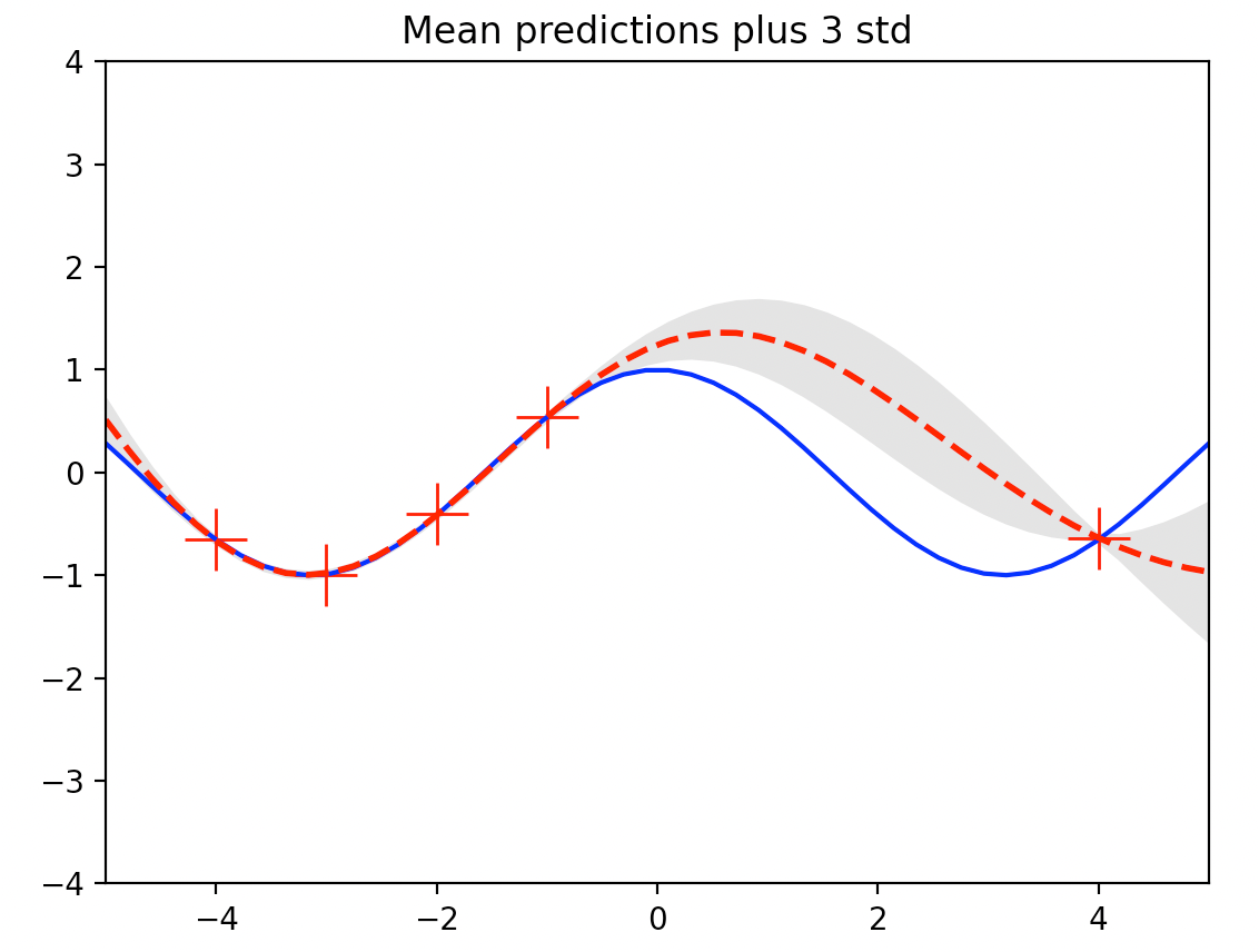
식 (8)로 계산한 테스트 입력
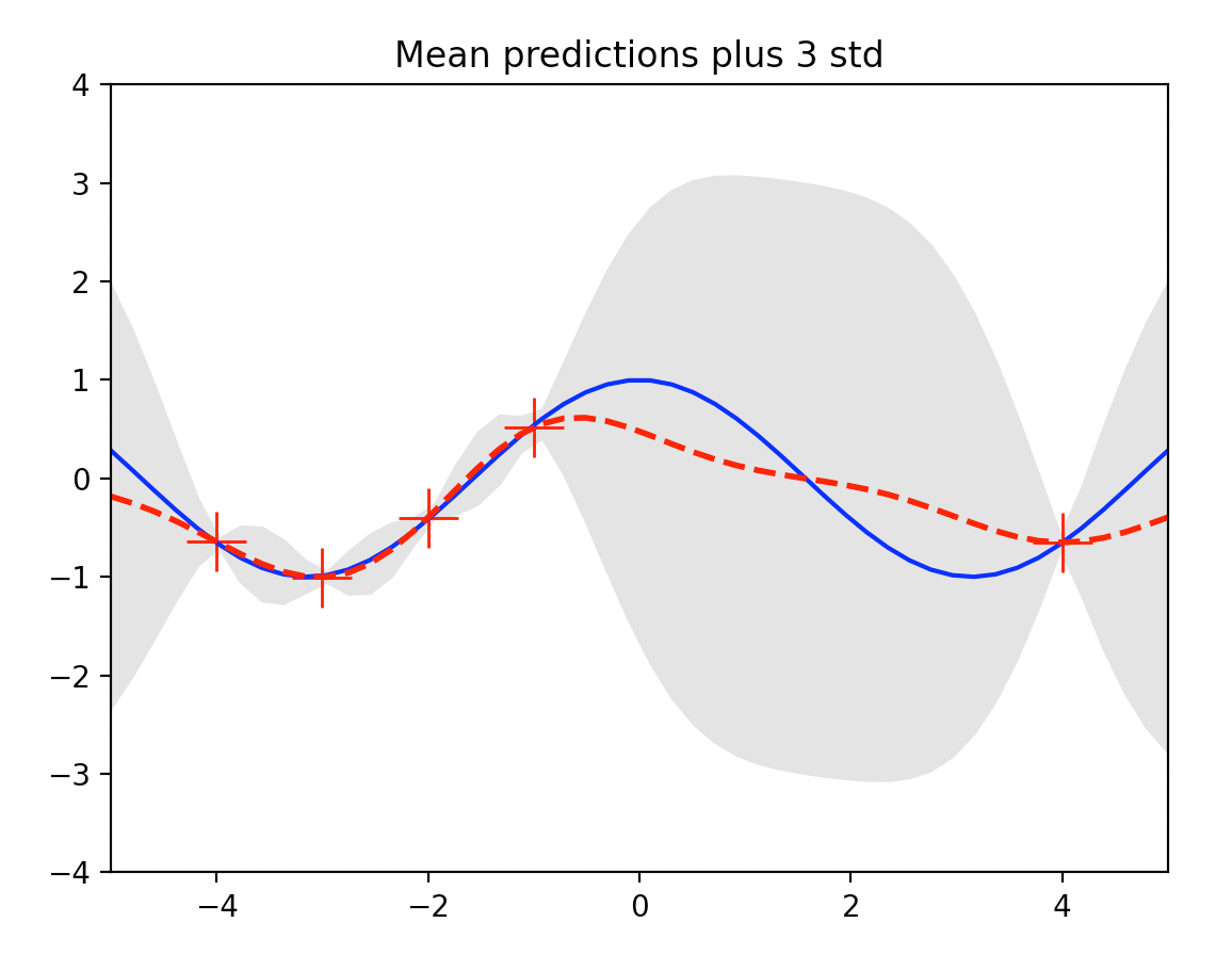
데이터가 밀집된 영역 (
다음 그림은 평균함수가
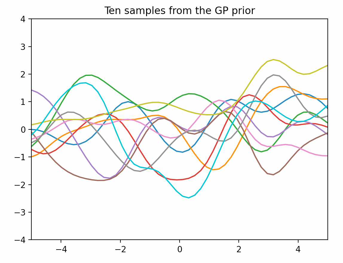
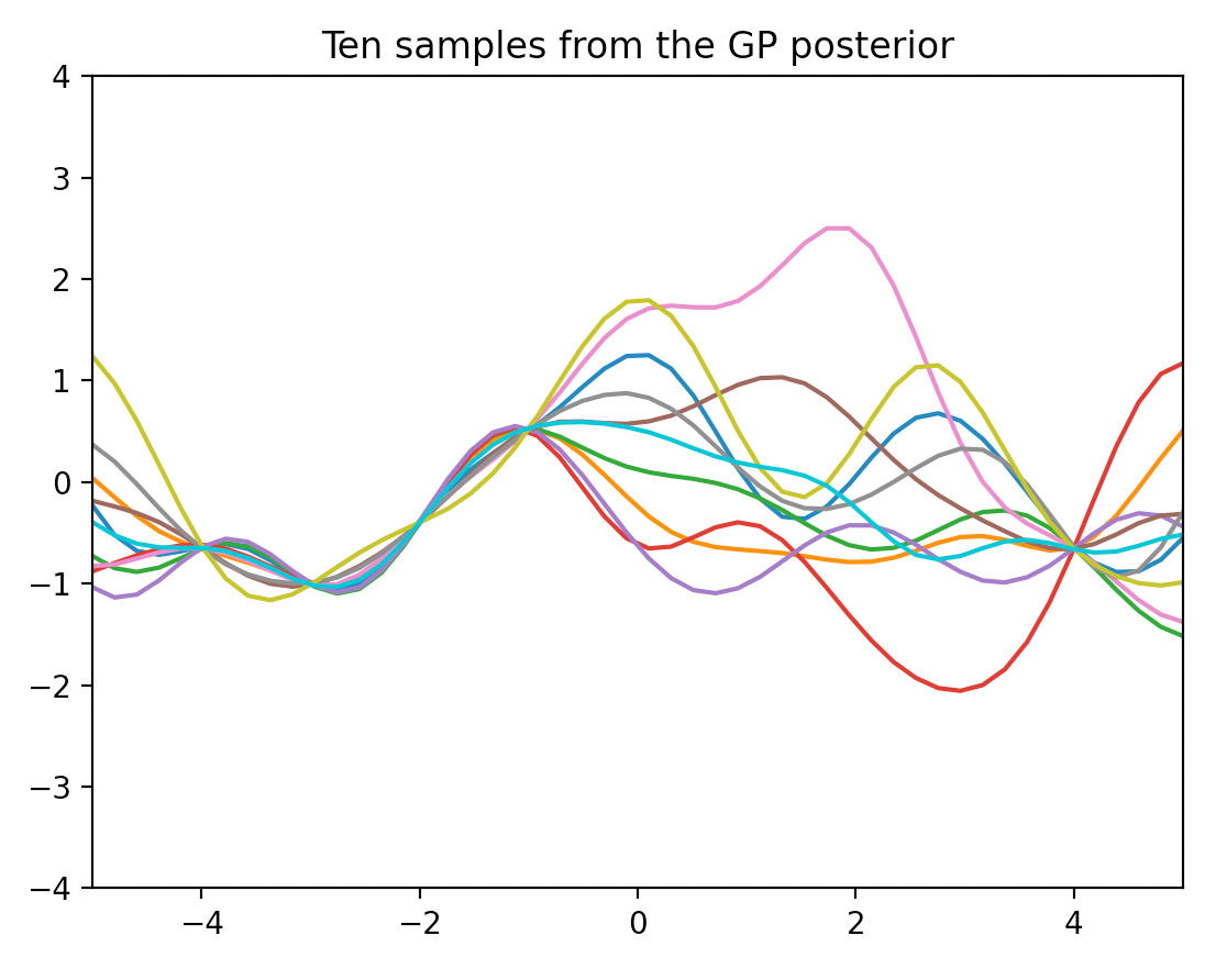
다음 그림은 식 (8)로 계산된 평균함수와 공분산을 갖는 가우시안 프로세스에서 10개의 샘플함수를 추출하여 그린 것이다. 데이터셋을 이용하여 GP prior를 업데이트 하여 얻은 프로세스이므로 사후 프로세스 (GP posterior) 라고 한다.
다음 그림은 커널 식 (7)에서
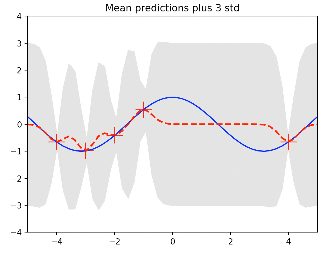
다음 그림은
다음은 본 예제에서 사용한 GP regression 의 전체 코드다.
# GP regression example
# by st.watermelon

import numpy as np
import matplotlib.pyplot as plt

# kernel
def kernel(a, b):
    lam2 = 1
    sqdist = np.sum(a**2,1).reshape(-1,1) + np.sum(b**2,1) - 2*np.dot(a, b.T)
    return np.exp(-.5 * sqdist / lam2)

# true function
f = lambda x: np.cos(x).flatten()

# parameters
p = 50         # number of test points
s = 0.01       # noise std

# training points (given)
X = np.array([ [-4], [-3], [-2], [-1], [4] ])
m = X.shape[0]  # number of training points
y = f(X) + s*np.random.randn(m)  #(m,)

K = kernel(X, X)
L = np.linalg.cholesky(K + s**2*np.eye(m))

# points for prediction
Xstar = np.linspace(-5, 5, p).reshape(-1,1)

# posterior mean (mu)
Kstar = kernel(X, Xstar)
Lstar = np.linalg.solve(L, Kstar)
mu_pos = np.dot(Lstar.T, np.linalg.solve(L, y))

# posterior covariance
K2star = kernel(Xstar, Xstar)
Sig = K2star - np.dot(Lstar.T, Lstar)

s2 = np.diag(Sig)
s = np.sqrt(s2)

# plotting
plt.figure(1)
plt.clf()
plt.plot(X, y, 'r+', ms=20)
plt.plot(Xstar, f(Xstar), 'b-')
plt.gca().fill_between(Xstar.flat, mu_pos-3*s, mu_pos+3*s, color="#dddddd")
plt.plot(Xstar, mu_pos, 'r--', lw=2)
plt.title('Mean predictions plus 3 std')
plt.axis([-5, 5, -4, 4])


# samples from the prior
L = np.linalg.cholesky(K2star + 1e-6*np.eye(p))
f_prior = np.dot(L, np.random.normal(size=(p,10)))
plt.figure(2)
plt.clf()
plt.plot(Xstar, f_prior)
plt.title('Ten samples from the GP prior')
plt.axis([-5, 5, -4, 4])


# samples from the posterior
L = np.linalg.cholesky(K2star + 1e-6*np.eye(p) - np.dot(Lstar.T, Lstar))
f_post = mu_pos.reshape(-1,1) + np.dot(L, np.random.normal(size=(p,10)))
plt.figure(3)
plt.clf()
plt.plot(Xstar, f_post)
plt.title('Ten samples from the GP posterior')
plt.axis([-5, 5, -4, 4])

plt.show()
'AI 딥러닝 > ML' 카테고리의 다른 글
| [GP-4] 베이지안 최적화 (Bayesian Optimization) (0) | 2022.07.09 |
|---|---|
| [GP-3] GP 커널 학습 (0) | 2022.07.05 |
| [GP-1] 가우시안 프로세스 (Gaussian Process)의 개념 (0) | 2022.06.26 |


댓글