Sequential API와 Functional API에 이어서 이번에는 Model Subclassing API를 이용하여 CNN을 구현해 보자.
Model Subclassing API는 자유도가 제일 높은 모델 구축 방법으로서 사용자 자신의 방법으로 신경망을 학습시킬 수도 있다. 딥러닝을 깊게 공부하려면 반드시 알아야 할 API다.
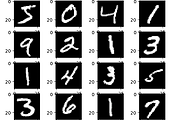
MNIST 숫자 분류 대신에 Fashion_MNIST 데이터셋을 이용해 보기로 한다. MNIST는 손글씨였지만 Fashion_MNIST는 신발, 가방, 옷 등의 흑백 그림을 모아 놓은 데이터셋이다.
텐서플로2에서는 Fashion_MNIST 데이터셋도 쉽게 다운로드할 수 있다.
fashion_mnist = tf.keras.datasets.fashion_mnist
(x_train, y_train), (x_test, y_test) = fashion_mnist.load_data()


# adjusting to 0 ~ 1.0
x_train = x_train / 255.0
x_test = x_test / 255.0
이미지를 몇 개 출력해 보면 다음과 같다.
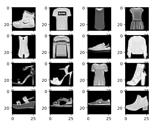
Fashion_MNIST의 라벨은 10가지로서 0: 상의, 1: 바지, 2: 스웨터, 3: 드레스, 4: 코트, 5: 샌달, 6: 셔츠, 7: 운동화, 8: 가방, 9: 부츠 등이다.
x_train와 x_test의 사이즈를 보면,
print(x_train.shape, x_test.shape)
(60000, 28, 28) (10000, 28, 28) 이다. 각각 데이터 개수가 6만개, 1만개이며 사이즈가 28x28 인 흑백 이미지다. CNN의 컨볼루션 레이어는 채널을 가진 데이터형을 받기 때문에 shape를 바꿔준다.
x_train = x_train.reshape(-1,28,28,1)
x_test = x_test.reshape(-1,28,28,1)
만들고자 하는 CNN 모델은 전과 똑같다.
2020/07/17 - [TensorFlow2] - TensorFlow2로 간단한 CNN 구현해 보기

Model Subclassing API를 사용하여 모델을 만들면 다음과 같다.
class MyModel(tf.keras.Model):
  def __init__(self):
    super(MyModel, self).__init__()
    self.conv1 = tf.keras.layers.Conv2D(kernel_size=(3,3), filters=16, activation='relu')
    self.conv2 = tf.keras.layers.Conv2D(kernel_size=(3,3), filters=32, activation='relu')
    self.conv3 = tf.keras.layers.Conv2D(kernel_size=(3,3), filters=64, activation='relu')
    self.pool = tf.keras.layers.MaxPooling2D((2, 2))
    self.flatten = tf.keras.layers.Flatten()
    self.d1 = tf.keras.layers.Dense(32, activation='relu')
    self.d2 = tf.keras.layers.Dense(10, activation='softmax')

  def call(self, x):
    x = self.conv1(x)
    x = self.pool(x)
    x = self.conv2(x)
    x = self.pool(x)
    x = self.conv3(x)
    x = self.flatten(x)
    x = self.d1(x)
    return self.d2(x)

model = MyModel()
여기서 __init__(self)는 객체가 생성될 때 호출되는 함수이고, call(self)는 객체 변수를 실행할 때 호출되는 함수다.
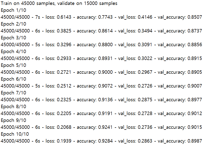
모델을 컴파일하고, MNIST보다 어려운 문제이므로 에폭 10으로 학습한다.
model.compile(optimizer='adam',
              loss='sparse_categorical_crossentropy',
              metrics=['accuracy'])


history = model.fit(x_train, y_train, epochs=10, validation_split=0.25)
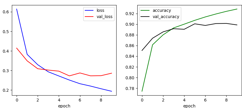
결과를 그림으로 그리면 다음과 같다.
plt.figure(figsize=(10,4))
plt.subplot(1,2,1)
plt.plot(history.history['loss'], 'b-', label='loss')
plt.plot(history.history['val_loss'], 'r-', label='val_loss')
plt.xlabel('epoch')
plt.legend()

plt.subplot(1,2,2)
plt.plot(history.history['accuracy'], 'g-', label='accuracy')
plt.plot(history.history['val_accuracy'], 'k-', label='val_accuracy')
plt.xlabel('epoch')
plt.legend()

plt.show()
학습된 모델을 테스트 데이터를 이용하여 평가해 보면,
test_loss, test_acc = model.evaluate(x_test, y_test)

print(test_acc)
0.891로서 약 89.1%의 테스트 정확도가 나온다.
전체 코드는 다음과 같다.
import tensorflow as tf
import matplotlib.pyplot as plt

# load fashion_mnist data
fashion_mnist = tf.keras.datasets.fashion_mnist
(x_train, y_train), (x_test, y_test) = fashion_mnist.load_data()


# adjusting to 0 ~ 1.0
x_train = x_train / 255.0
x_test = x_test / 255.0

print(x_train.shape, x_test.shape)

# reshaping
x_train = x_train.reshape(-1,28,28,1)
x_test = x_test.reshape(-1,28,28,1)

# plotting
plt.figure()
for c in range(16):
    plt.subplot(4,4,c+1)
    plt.imshow(x_train[c].reshape(28,28), cmap='gray')
plt.show()

class MyModel(tf.keras.Model):
  def __init__(self):
    super(MyModel, self).__init__()
    self.conv1 = tf.keras.layers.Conv2D(kernel_size=(3,3), filters=16, activation='relu')
    self.conv2 = tf.keras.layers.Conv2D(kernel_size=(3,3), filters=32, activation='relu')
    self.conv3 = tf.keras.layers.Conv2D(kernel_size=(3,3), filters=64, activation='relu')
    self.pool = tf.keras.layers.MaxPooling2D((2, 2))
    self.flatten = tf.keras.layers.Flatten()
    self.d1 = tf.keras.layers.Dense(32, activation='relu')
    self.d2 = tf.keras.layers.Dense(10, activation='softmax')

  def call(self, x):
    x = self.conv1(x)
    x = self.pool(x)
    x = self.conv2(x)
    x = self.pool(x)
    x = self.conv3(x)
    x = self.flatten(x)
    x = self.d1(x)
    return self.d2(x)

model = MyModel()

# compile and train
model.compile(optimizer='adam',
              loss='sparse_categorical_crossentropy',
              metrics=['accuracy'])


history = model.fit(x_train, y_train, epochs=10, validation_split=0.25)

plt.figure(figsize=(10,4))
plt.subplot(1,2,1)
plt.plot(history.history['loss'], 'b-', label='loss')
plt.plot(history.history['val_loss'], 'r-', label='val_loss')
plt.xlabel('epoch')
plt.legend()

plt.subplot(1,2,2)
plt.plot(history.history['accuracy'], 'g-', label='accuracy')
plt.plot(history.history['val_accuracy'], 'k-', label='val_accuracy')
plt.xlabel('epoch')
plt.legend()

plt.show()

# model evaluate
test_loss, test_acc = model.evaluate(x_test, y_test)

print(test_acc)
'프로그래밍 > TensorFlow2' 카테고리의 다른 글
| 텐서와 변수 - 2 (0) | 2021.02.10 |
|---|---|
| 텐서와 변수 - 1 (0) | 2021.02.09 |
| GradientTape로 간단한 CNN 학습하기 (0) | 2021.01.11 |
| Functional API로 간단한 CNN 구현해 보기 (0) | 2021.01.11 |
| Sequential API로 간단한 CNN 구현해 보기 (0) | 2020.07.17 |


댓글